6.3 Riemann Sums, Summation Notation, and Definite Integral Notation

TLDR

A definite integral is the exact limit of a Riemann sum as the rectangle widths shrink to zero. In AP Calculus, this topic is about writing a Riemann sum in summation notation, recognizing the limit of that sum as $\int_a^b f(x)\, dx$, and translating back and forth between the two forms.

Riemann Sums and Definite Integral Notation Summary

Riemann sums approximate accumulated area or change by adding products of function values and subinterval widths. A definite integral represents the limiting case of those Riemann sums as the subinterval widths approach zero.

For AP Calculus, you need to translate both directions: from a Riemann sum or summation notation into a definite integral, and from a definite integral into the related limiting Riemann sum. Track the interval, subinterval width, sample point, integrand, and limits of integration carefully.

Why This Matters for the AP Calculus Exam

Unit 6 carries a lot of weight on the AP Calculus exam, and this topic is the bridge that turns approximation into exact area. Once you see that a definite integral is just a Riemann sum pushed to the limit, the Fundamental Theorem of Calculus in later topics makes much more sense.

On the exam you may be asked to:

• Match a given limit of a Riemann sum to the correct definite integral, or vice versa.
• Set up a Riemann sum from a function, interval, and number of subintervals.
• Interpret the sum of products (function value times subinterval width) as accumulated change or signed area.

Being precise with notation matters for clear exam work, especially the integrand, the limits of integration, and the differential $dx$.

Key Takeaways

• A Riemann sum splits an interval into subintervals and adds up products of a function value times a subinterval width: $\sum_{i=1}^{n} f(x_i^*)\,\Delta x_i$.
• The definite integral is the limit of those sums as the widths shrink: $\int_a^b f(x)\, dx = \lim_{\max \Delta x_i \to 0} \sum_{i=1}^{n} f(x_i^*)\,\Delta x_i$.
• With equal subintervals, $\Delta x = \frac{b-a}{n}$, and the limit can be written as $n \to \infty$.
• For a right Riemann sum with equal widths, $x_i = a + \Delta x \cdot i$.
• You should be able to go both directions: turn a definite integral into the limit of a Riemann sum, and read a limit of a sum as a definite integral.
• The result is exact, not an approximation, once you take the limit.

Summation Notation

Before connecting to integrals, you need a faster way to write a Riemann sum. Summation notation lets you use algebra instead of adding each rectangle by hand.

Consider $f(x) = x^2$ over the interval from 0 to 5.

Desmos graph of $f(x) = x^2$ with area under the curve from $[0,5]$ shaded.

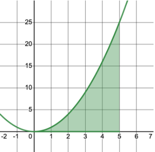
Use a left Riemann sum with 5 subintervals to approximate the area.

The same Desmos graph with 5 left-endpoint Riemann rectangles.

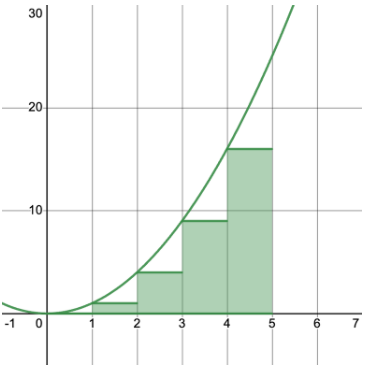
To convert this to summation notation, build a function that gives the area of each rectangle. Call it $A$, so $A(i)$ gives the area of the $i$th rectangle:

$$\sum_{i=0}^{4}A(i)$$

The area of each rectangle is $b\cdot h$, where $b$ is the base width and $h$ is the height.

The base width is constant. Divide the whole interval by the number of subintervals:

$$\frac{5-0}{5}=1$$

The height is the value of $f$ at each left endpoint. To find the $i$th x-value, start at 0 and add 1 (the subinterval width) repeatedly.

A graph showing the relationship between the subinterval length and $x_i$.

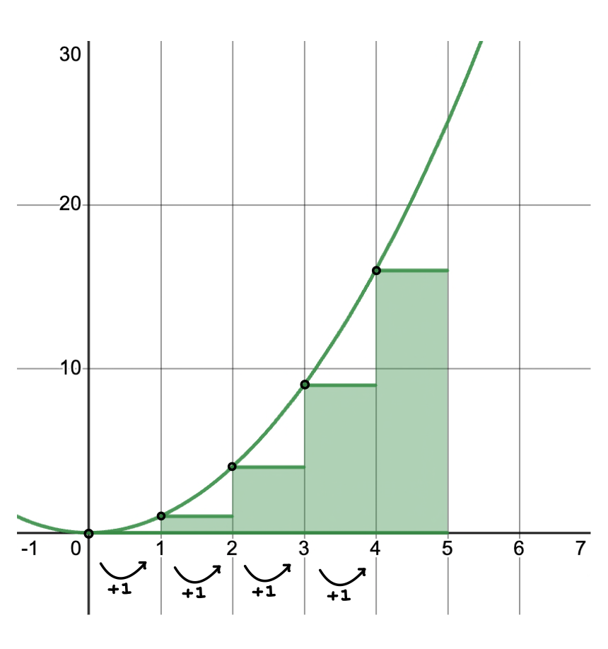
The x-value is $1i$, or just $i$. Plug it into the function to get the height: $y_i=(i)^2$. Combine these in the area formula:

$$A(i)=1\cdot i^2$$

which simplifies to

$$A(i)=i^2$$

Plug that into the summation:

$$\sum_{i=1}^{5}i^2$$

General Form of a Riemann Sum

The general form in summation notation is:

$$\sum_{i=0}^{n-1} {\Delta x}\cdot{f({x_i})}$$

for left endpoints, and

$$\sum_{i=1}^{n} {\Delta x}\cdot{f({x_i})}$$

for right endpoints.

Here is what each symbol means:

• $n$: the number of subintervals, usually given in the problem.
• $a$: the lower bound of the interval.
• $b$: the upper bound of the interval.
• $\Delta x$: the width of each subinterval, found with $\frac{b-a}{n}$.
• $x_i$: the right endpoint of each rectangle, $x_i=a+\Delta x\cdot i$.
• $f(x_i)$: the original function with $x_i$ plugged in.
• $\sum$: add up the values from $0\rightarrow n-1$ for left Riemann sums or $1\rightarrow n$ for right Riemann sums.

Connecting to Definite Integrals

In the last topic you saw that a Riemann sum gets more precise as you use more rectangles, meaning a larger $n$. What if you had infinitely many rectangles with infinitely tiny widths?

GIF illustrating the left Riemann sum as $n$ grows. GIF courtesy of Maplesoft

As $n\rightarrow \infty$, the approximation gets closer and closer to the exact area. That connects the Riemann sum to the definite integral:

$$\lim_{n\to \infty}\sum_{i=1}^{n} {\Delta x}\cdot{f({x_i})}=\int_a^bf(x)\ dx$$

where $\Delta x=\frac{b-a}{n}$ and $x_i=a+\Delta x\cdot i$.

This limit gives the exact value of the definite integral, not just an approximation.

Walkthrough

Given $f(x)=x^2+3$ over $[0,5]$, write the summation notation for the right Riemann sum with 10 subintervals and find its value. Then write the definite integral as the limit of the right Riemann sum as $n$ approaches infinity.

1) Summation Notation

Write the general form first:

$$\sum_{i=1}^{10}\Delta x\cdot f(x_i)$$

Define $\Delta x=\frac{b-a}{n}=\frac{5-0}{10}=0.5$. Then $x_i=a+\Delta x\cdot i=0.5i$. Plug into the function: $f(x_i)=(0.5i)^2+3$. The right Riemann sum with 10 subintervals is:

$$\sum_{i=1}^{10}0.5\cdot \big((0.5i)^2+3\big)$$

To calculate it, plug in $i=1$ through $10$ and add:

$$0.5(3.5+5+7.5+11+15.5+21+27.5+35+43.5+53)=\boxed{111.25}$$

2) Writing the Definite Integral

First write the definite integral:

$$\int_0^5 x^2+3\ dx$$

Recall the general form:

$$\lim_{n\to \infty}\sum_{i=1}^{n} {\Delta x}\cdot{f({x_i})}=\int_a^bf(x)\ dx$$

Since $n$ is the limit variable, define every term in terms of $n$:

1. $\Delta x=\frac{5-0}{n}=\frac{5}{n}$.
2. $x_i=a+\Delta x\cdot i=0+\frac{5}{n}\cdot i=\frac{5}{n}i$.
3. $f(x_i)=\left(\frac{5}{n}i\right)^2+3$.

Put it together:

$$\int_0^5x^2+3\ dx=\lim_{n\to \infty}\sum_{i=1}^{n} \frac{5}{n}\cdot \Bigg[ \Big( \frac{5}{n} i\Big)^2+3\Bigg]$$

These take practice, but once finding $\Delta x$ and $x_i$ becomes automatic, they get very doable.

How to Use This on the AP Calculus Exam

Problem Solving

When you convert a definite integral into the limit of a Riemann sum, use the same steps every time:

1. Find $\Delta x = \frac{b-a}{n}$.
2. Find $x_i = a + \Delta x \cdot i$.
3. Substitute $x_i$ into the function to get $f(x_i)$.
4. Assemble $\lim_{n\to\infty}\sum_{i=1}^{n} \Delta x \cdot f(x_i)$.

MCQ

A common multiple-choice task gives you a limit of a sum and asks for the matching definite integral, or the reverse. Read the pieces: the factor that looks like $\frac{b-a}{n}$ is your $\Delta x$, and the expression inside the function tells you $x_i$, which reveals $a$, $b$, and the function. Break the complicated expression into familiar parts instead of trying to read it all at once.

Common Trap

Watch parentheses carefully when you substitute $x_i$ into a function with a square or other power. Writing $\frac{5}{n}i^2$ when you mean $\left(\frac{5}{n}i\right)^2$ changes the answer.

Riemann Sum Practice

Try these three, then check the solutions.

Practice Problems

1. For $f(x)=4x^2+2x-1$, express $\int_1^3 f(x)\ dx$ as the limit of a Riemann sum.
2. Express $\int_0^2 2e^x+1 \ dx$ as the limit of a Riemann sum.
3. The velocity function is $v(t)=2t+1$ on the interval $[1,4]$. Express $\int_1^4 v(t)\ dt$ as the limit of a Riemann sum.

Solutions

Practice Problem 1

Define $\Delta x=\frac{3-1}{n}=\frac{2}{n}$. Then $x_i=a+\Delta x\cdot i=1+\frac{2}{n}i$. Plug into $f(x)$:

$$f(x_i)=4\left(1+\frac{2}{n}i\right)^2+2\left(1+\frac{2}{n}i\right)-1$$

Assemble:

$$\int_1^3f(x)\ dx=\lim_{n\to \infty}\sum_{i=1}^n \frac{2}{n}\cdot \Bigg(4\left(1+\frac{2}{n}i\right)^2+2\left(1+\frac{2}{n}i\right)-1\Bigg)$$

Practice Problem 2

Define $\Delta x=\frac{2-0}{n}=\frac{2}{n}$. Then $x_i=a+\Delta x\cdot i=\frac{2}{n}i$. Plug into $f(x)$:

$$f(x_i)=2e^{2i/n}+1$$

Assemble:

$$\int_0^2f(x)\ dx=\lim_{n\to \infty}\sum_{i=1}^n \frac{2}{n}\cdot (2e^{2i/n}+1)$$

Practice Problem 3

Define $\Delta t=\frac{4-1}{n}=\frac{3}{n}$. Then $t_i=a+\Delta t\cdot i=1+\frac{3}{n}i$. Plug into $v(t)$:

$$v(t_i)=2\left(1+\frac{3}{n}i\right)+1=2+\frac{6}{n}i+1=\frac{6}{n}i+3$$

Assemble:

$$\int_1^4v(t)\ dt=\lim_{n\to \infty}\sum_{i=1}^n \frac{3}{n}\cdot \left(\frac{6}{n}i+3\right)$$

Common Misconceptions

• The definite integral is not an approximation. A Riemann sum with a fixed $n$ approximates, but once you take the limit, the value is exact.
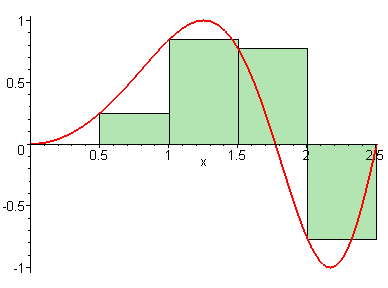
• A Riemann sum is not just "the area." It is a sum of products of function value times subinterval width, and it gives signed area, so regions below the x-axis count as negative.
• $x_i^*$ does not have to be a left or right endpoint. The sample point can be anywhere in the subinterval, including the midpoint. For continuous functions on $[a,b]$, the limit comes out the same.
• $\Delta x = \frac{b-a}{n}$ only when the subintervals are equal in width. With a nonuniform partition, each $\Delta x_i$ can differ, which is why the general definition uses $\max \Delta x_i \to 0$.
• Do not drop the $dx$ when writing a definite integral. The differential shows the variable of integration and is part of correct notation.

Related AP Calculus Guides

• Unit 6 Overview: Integration and Accumulation of Change
• 6.11 Integrating Using Integration by Parts
• 6.1 Integration and Accumulation of Change
• 6.12 Integrating Using Linear Partial Fractions
• 6.4 The Fundamental Theorem of Calculus and Accumulation Functions
• 6.5 Interpreting the Behavior of Accumulation Functions Involving Area