5.9 Connecting a Function, Its First Derivative, and its Second Derivative

The graphs of a function $f$, its first derivative $f'$, and its second derivative $f''$ are all linked. The sign of $f'$ tells you where $f$ is increasing or decreasing, the sign of $f''$ tells you concavity, and the places where $f'$ or $f''$ cross the x-axis point to extrema and inflection points. For AP Calculus, name which graph you are using before making a conclusion about $f$.

Why This Matters for the AP Calculus Exam

This topic pulls together everything from earlier in Unit 5 and asks you to reason graphically instead of only algebraically. On the AP Calculus exam, you often get the graph of $f'$ (or sometimes $f''$) and have to draw conclusions about $f$ without ever seeing a formula. That shows up in both multiple-choice questions and free-response questions, where you may need to justify where $f$ has a maximum, a minimum, or a point of inflection.

The justifications you write here matter for clear exam work. Reasoning like "$f$ is concave up on this interval because $f'$ is increasing there" is exactly the kind of language graders look for. Refer to $f$, $f'$, and $f''$ by name, not "it" or "the function," so your argument is easy to follow.

Key Takeaways

• Where $f'$ is positive, $f$ is increasing; where $f'$ is negative, $f$ is decreasing.
• Where $f''$ is positive, $f$ is concave up and $f'$ is increasing; where $f''$ is negative, $f$ is concave down and $f'$ is decreasing.
• Relative extrema of $f$ happen where $f'$ crosses the x-axis (changes sign).
• Points of inflection of $f$ line up with relative extrema of $f'$ and with sign changes of $f''$.
• A critical point occurs where $f'=0$ or $f'$ does not exist (such as a cusp or vertical tangent).
• The First and Second Derivative Tests both work in graphical form, not just algebraic form.

Connecting the Three Graphs

Given the graphs of $f$, $f'$, and $f''$, or just one of them, you can read off information about the others. Instead of using equations, you look at where a graph crosses the x-axis, where it is positive or negative, and where it is increasing or decreasing.

Guides worth revisiting before this one:

• 5.3 Determining Intervals on Which a Function Is Increasing or Decreasing
• 5.4 Using the First Derivative Test to Determine Relative (Local) Extrema
• 5.6 Determining Concavity of Functions over Their Domains
• 5.7 Using the Second Derivative Test to Determine Extrema

Trends and Concavity

Here is a quick summary of how the three graphs connect:

• When $f$ is increasing, $f'$ is positive ($>0$).
• When $f$ is decreasing, $f'$ is negative ($<0$).
• When $f$ is concave up, $f''$ is positive ($>0$) and $f'$ is increasing.
• When $f$ is concave down, $f''$ is negative ($<0$) and $f'$ is decreasing.

Apply this to the graph of a function $g(x)$ below.

Graph of function $g(x)$, courtesy of Zweig Media

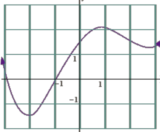
Describing $g'(x)$ across intervals:

• On $(-\infty,-2)$ and $(0.85,2.8)$, $g(x)$ is decreasing, so $g'(x)$ is negative.
• On $(-2, 0.85)$ and $(2.8,\infty)$, $g(x)$ is increasing, so $g'(x)$ is positive.

Now describing $g''(x)$ using concavity:

• On $(-\infty,-0.5)$ and $(1.5, \infty)$, $g(x)$ is concave up, so $g''(x)$ is positive and $g'(x)$ is increasing.
• On $(-0.5,1.5)$, $g(x)$ is concave down, so $g''(x)$ is negative and $g'(x)$ is decreasing.

Extrema and Points of Inflection

Where the graph of $f$ changes direction or concavity, you can pin down maxima, minima, x-intercepts, and inflection points on the graphs of $f'$ and $f''$.

• If $f(x)$ has a relative minimum (changes from decreasing to increasing), then $f'(x)$ changes from negative to positive there.
• If $f(x)$ has a relative maximum (changes from increasing to decreasing), then $f'(x)$ changes from positive to negative there.
• If $f(x)$ has a point of inflection going from concave up to concave down, then $f'(x)$ has a relative maximum and $f''(x)$ changes from positive to negative there.
• If $f(x)$ has a point of inflection going from concave down to concave up, then $f'(x)$ has a relative minimum and $f''(x)$ changes from negative to positive there.

Two big ideas to remember:

1. All relative extrema of $f(x)$ are x-intercepts of $f'(x)$.
2. All points of inflection of $f(x)$ are relative extrema of $f'(x)$.

How to Use This on the AP Calculus Exam

Problem Solving

When you are handed a graph of $f'$, read it like a sign chart. Find where it crosses the x-axis, then check whether it goes from negative to positive (relative minimum of $f$) or positive to negative (relative maximum of $f$). This is the First Derivative Test in graphical form.

When you are handed a graph of $f''$, check its sign to find concavity, and find where it crosses the x-axis (and changes sign) to locate inflection points of $f$.

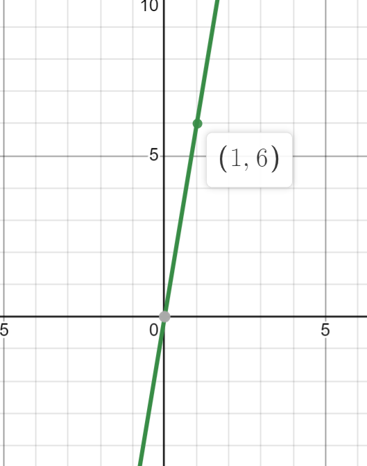
Worked Example: Reading a Graph of $f'$

The derivative $f'$ of the differentiable function $f$ is graphed below.

Graph of the derivative of $f$ with the point $(1.5, 0)$ labeled. Image created with Desmos.

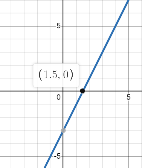
What happens to $f$ at $x=1.5$?

The graph of $f'$ crosses the x-axis at $x=1.5$. It is negative before that point and positive after it, so $f$ is decreasing then increasing. That makes $x=1.5$ a relative minimum of $f$. This is just the First Derivative Test applied graphically.

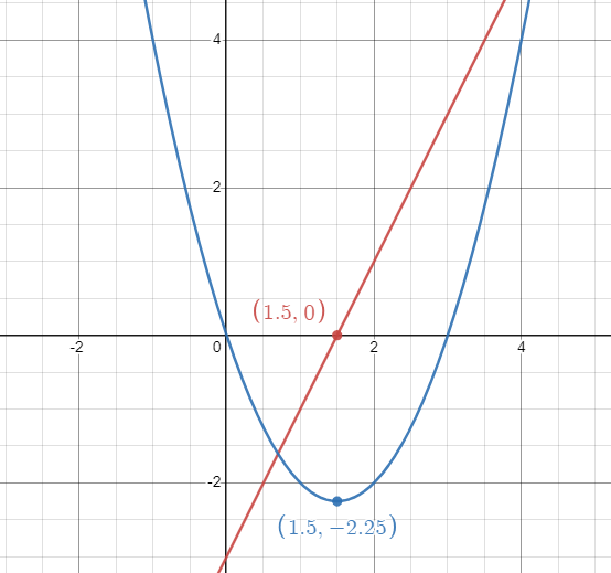
Here are $f(x)=x^2-3x$ and $f'(x)=2x-3$ together so you can see the connection.

Graph of $f(x)=x^2-3x$ and its derivative $f'(x)=2x-3$. Image created with Desmos.

Worked Example: Extrema and Inflection on One Graph

Returning to the graph of $g(x)$:

Graph of function $g(x)$. Image courtesy of Zweig Media.

• At $x=-2$ and $x=2.8$, $g(x)$ has relative minima, so $g'(x)$ has x-intercepts there and changes from negative to positive.
• At $x=0.85$, $g(x)$ has a relative maximum, so $g'(x)$ has an x-intercept and changes from positive to negative.
• At $x=-0.5$, $g(x)$ has a point of inflection (concave up to concave down), so $g'(x)$ has a relative maximum and $g''(x)$ has an x-intercept changing from positive to negative.
• At $x=1.5$, $g(x)$ has a point of inflection (concave down to concave up), so $g'(x)$ has a relative minimum and $g''(x)$ has an x-intercept changing from negative to positive.

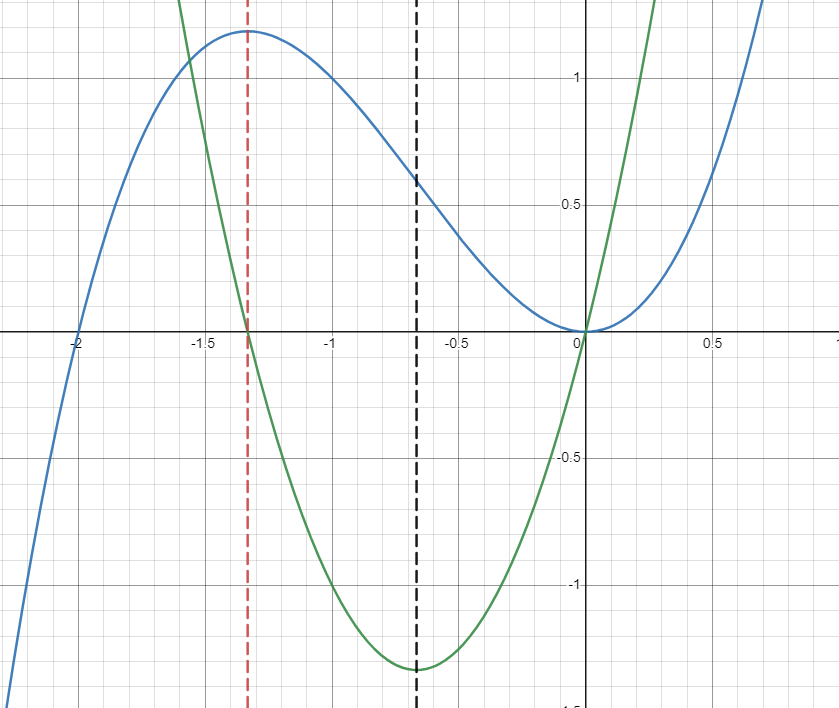
Worked Example: Cubic Function

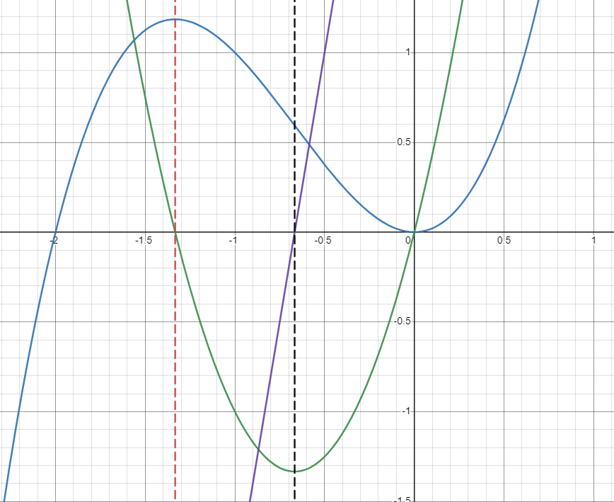
Look at the graph of $h(x)=x^3+2x^2$ and think about three things:

1. What happens to $h'(x)$ at $x=-1.3$ (red dotted line)?
2. What happens to $h'(x)$ at $x=-0.667$ (black dotted line)?
3. What happens to $h''(x)$ at $x=-0.667$?

Graph of $h(x)=x^3+2x^2$. Image created with Desmos.

At $x=-1.3$, $h(x)$ has a relative maximum, so $h'(x)$ has an x-intercept there and changes from positive to negative.

At $x=-0.667$, $h(x)$ changes from concave down to concave up, so $h'(x)$ has a relative minimum and $h''(x)$ has an x-intercept changing from negative to positive.

Here is $h(x)$ in blue and $h'(x)$ in green so you can see those trends.

Graph of $h(x)=x^3+2x^2$ and $h'(x)=3x^2+4x$. Image created with Desmos.

And here is the same graph with $h''(x)$ added in purple.

Graph of $h(x)=x^3+2x^2$, $h'(x)=3x^2+4x$, and $h''(x)=6x+4$. Image created with Desmos.

Practice Problems

Question 1:

The second derivative $f''$ of the differentiable function $f$ is graphed.

Graph of the second derivative of $f$ with the point $(1, 6)$ labeled. Image created with Desmos.

Given that $f'(1)=0$, what can you tell about $f$ at $x=1$ based on the graph of $f''$?

Question 2:

The second derivative $f''$ of the differentiable function $f$ is graphed.

Graph of the second derivative of $f$ with the point $(-1.8, 0)$ labeled. Image created with Desmos.

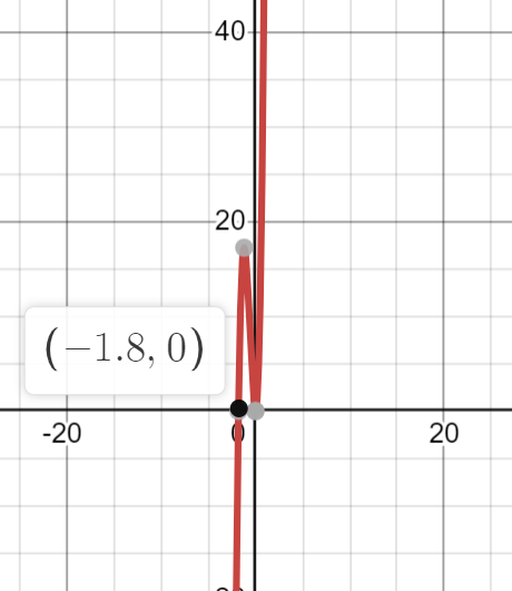
What can you tell about $f$ at $x=-2.4$ based on the graph of $f''$?

Answers and Solutions

Question 1:

Answer: $f$ has a relative minimum at $x=1$.

Solution: The graph of $f''$ is positive at $x=1$, so $f$ is concave up there. Combined with $f'(1)=0$, the Second Derivative Test tells you $f$ has a relative minimum at $x=1$.

Question 2:

Answer: $f$ is concave down at $x=-2.4$.

Solution: The graph of $f''$ is negative at $x=-2.4$, so $f$ is concave down there.

Common Misconceptions

• Treating features of the $f'$ graph as if they belong to $f$. If the graph of $f'$ is going up, that means $f$ is concave up, not that $f$ itself is increasing. Increasing $f$ comes from $f'$ being positive, not from $f'$ rising.
• Confusing an x-intercept of $f'$ with an inflection point. An x-intercept of $f'$ where $f'$ changes sign is a relative extremum of $f$. Inflection points of $f$ line up with extrema of $f'$, where $f''$ changes sign.
• Assuming every zero of $f'$ is a maximum or minimum. If $f'$ touches the x-axis but does not change sign, $f$ has no extremum there.
• Assuming every zero of $f''$ is an inflection point. An inflection point requires $f''$ to actually change sign, not just equal zero.
• Forgetting that critical points can come from $f'$ being undefined, such as at a cusp or vertical tangent, not only from $f'=0$.
• Using vague words like "it" in justifications. Always name $f$, $f'$, or $f''$ so your reasoning is clear.

Related AP Calculus Guides

• Unit 5 Overview: Analytical Applications of Differentiation
• 5.1 Using the Mean Value Theorem
• 5.2 Extreme Value Theorem, Global vs Local Extrema, and Critical Points
• 5.3 Determining Intervals on Which a Function is Increasing or Decreasing
• 5.4 Using the First Derivative Test to Determine Relative (Local) Extrema
• 5.11 Solving Optimization Problems