6.2 Approximating Areas with Riemann Sums
Welcome back to AP Calc with Fiveable! In the last guide, we explored accumulations of change and thought about how to compute them. Here, we’ll take a deep dive into Riemann sums, a method for approximating the area under the curve to find the accumulation of change.

📶 Graphical Riemann Sums
As we delve into integral calculus, our goal has shifted from computing the instantaneous rate of change to computing the area under the curve. Riemann sums are a useful tool for approximating this. Take a look at this graph:
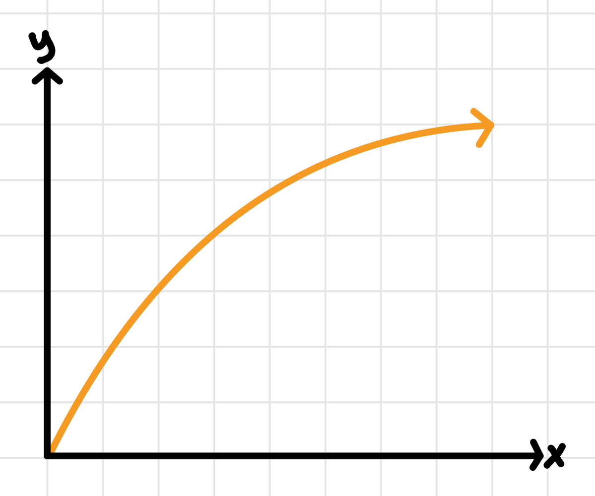
You would have a hard time computing this geometrically. But, we can approximate it using familiar shapes, like this:
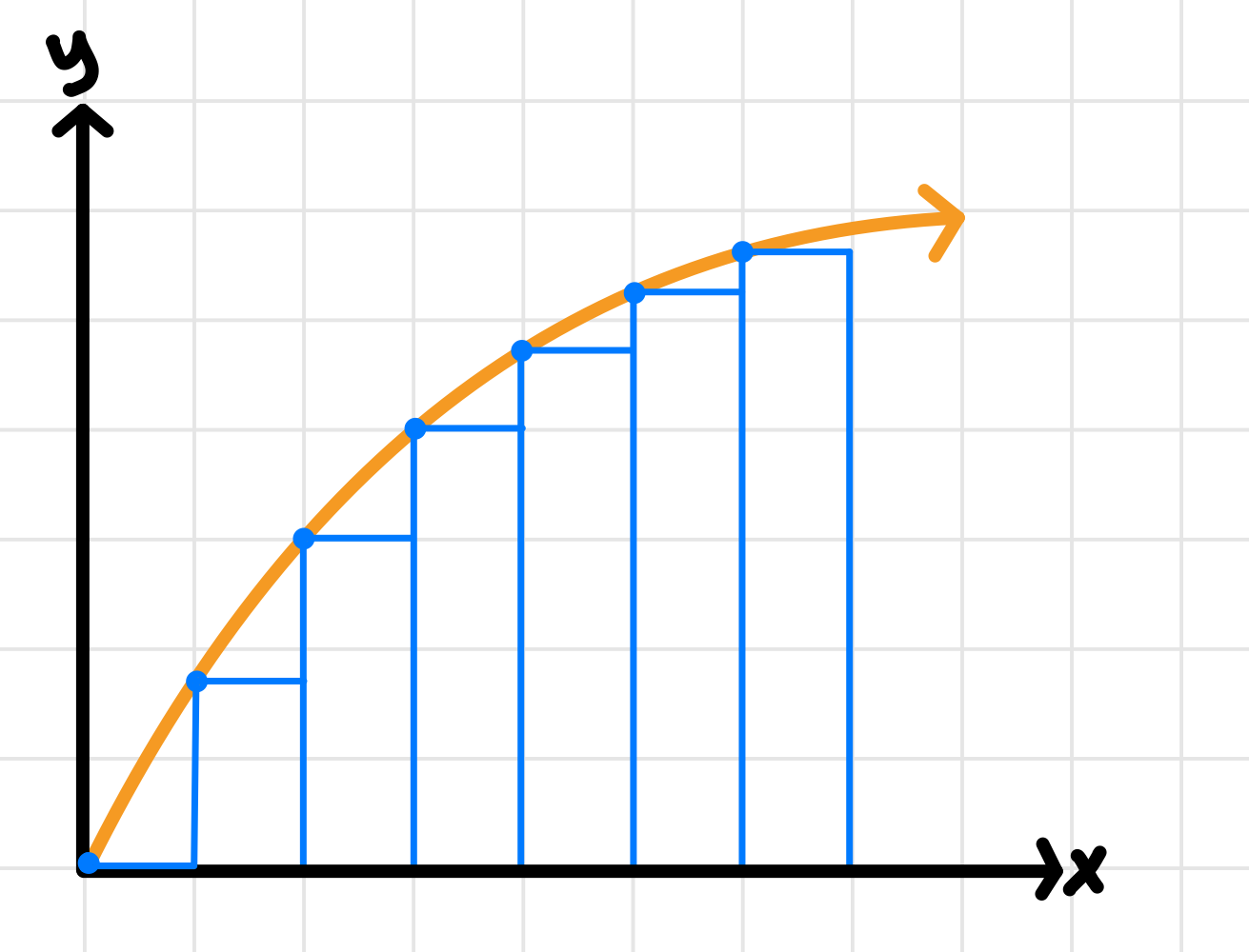
We can see that this isn’t exact, but that our approximation improves if we use more and more rectangles:
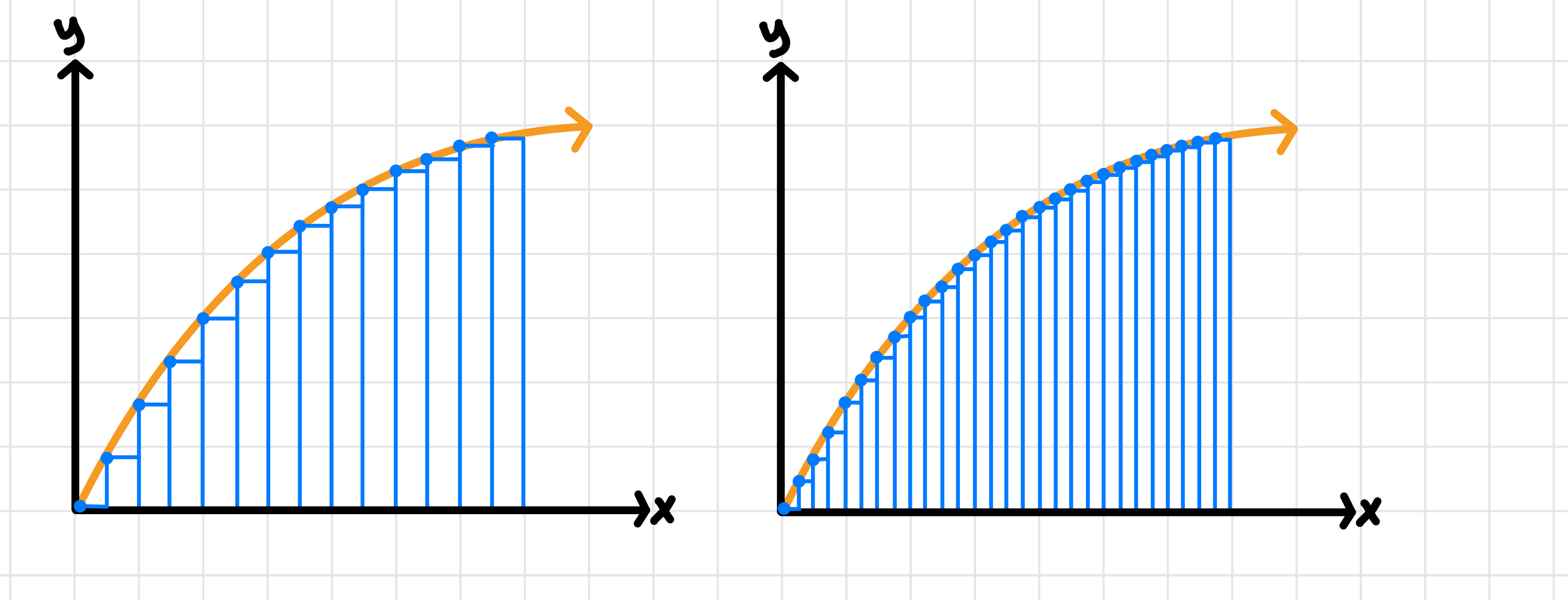
The use of these rectangles to approximate the area under the curve is called a Riemann sum. There are four main Riemann sums:
- Left Riemann Sum
- Right Riemann Sum
- Midpoint Riemann Sum
- Trapezoidal Sum
Now, let’s get into each of these in detail!
↔️ Left and Right Riemann Sum
There are two basic types of Riemann sums, called “left endpoint” and “right endpoint.” Here is an example of the same curve with a left Riemann sum, versus one with a right Riemann sum:

You can see that the left and right refer to which points we use to determine the height of our rectangles. Left Riemann sums touch the curve with their top left corners, and right Riemann sums touch the curve with their top right corners.
💡 Notation Tip: The left Riemann sum is notated like so: , where is the number of subdivisions. Likewise, the right Riemann sum is notated as .
➗ Subdivisions
Another thing that we can vary when deciding to take a Riemann sum is the width of our base. Our base length can either be uniform or non-uniform, as illustrated here:
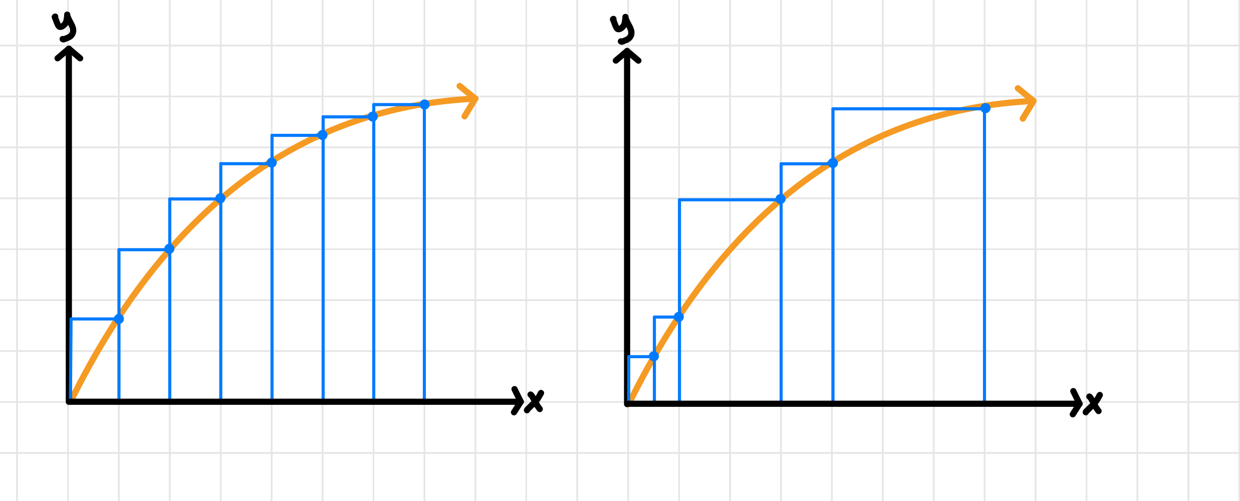
The base lengths formed by dividing up the total interval are called “subdivisions.”
🤔 Overestimating vs Underestimating
We know that a Riemann sum isn’t a perfect calculation of our area under the curve, but are we overestimating or underestimating when we use one? Try these problems and then fill in the blanks to see if you can figure out the pattern!
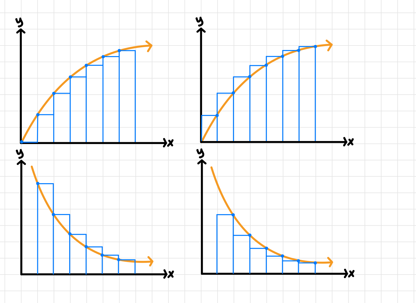
Fill in the Blanks! 🧠
- A left Riemann sum ________when a function is ________.
- A right Riemann sum ________when a function is ________.
- A left Riemann sum ________when a function is ________.
- A right Riemann sum ________when a function is ________.
⚡ Answer Key:
If you haven’t already guessed the pattern, here are the rules:
- A left Riemann sum underestimates when a function is increasing 📈
- A right Riemann sum overestimates when a function is increasing 📈
- A left Riemann sum overestimates when a function is decreasing 📉
- A right Riemann sum underestimates when a function is decreasing 📉
Now that we know which types of Riemann sums make which types of errors in their estimations, how might we make our approximation more accurate?
📐 Trapezoidal and Midpoint Riemann Sums
If you guessed by averaging the two estimations, you’d be correct! We can do this in one of two ways.
📐 Trapezoidal Riemann Sum
If you’ve already calculated the left and right Riemann sum for a graph, you can simply take their average. But, there’s an even faster way to do this, using another simple geometric shape—the trapezoid! Instead of finding just the left or right endpoints, we mark every point over the interval we’re interested in. Then, we connect pairs of points together:

This creates trapezoids! Instead of using the area formula for a rectangle, we now take the average of the two side lengths and multiple them by the base, using this formula:
💡 Notation Tip: The trapezoidal Riemann sum is notated like so: , where is the number of subdivisions.
📍 Midpoint Riemann Sum
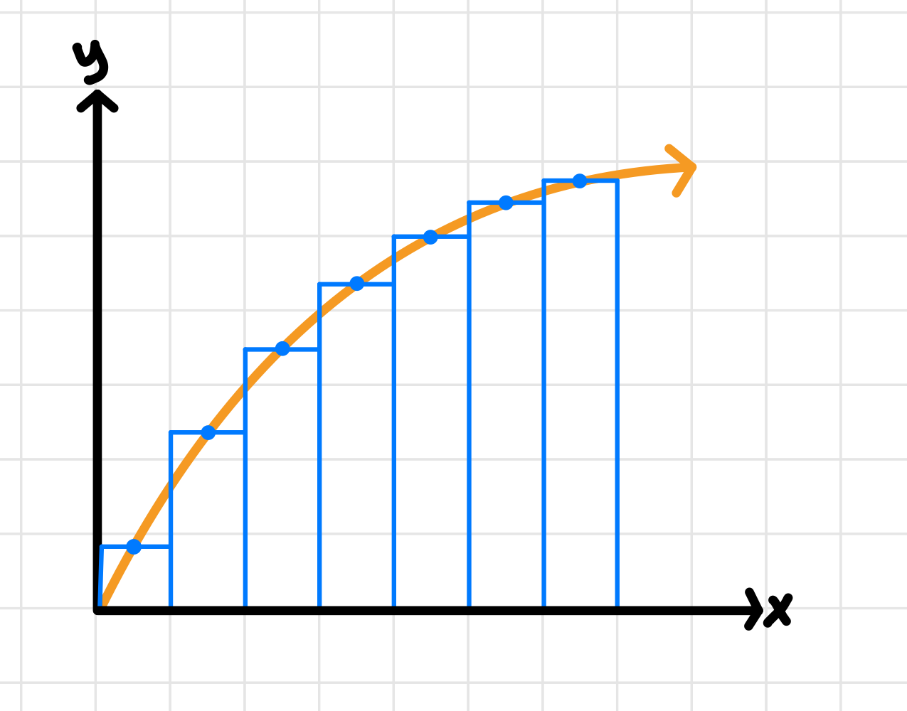
Midpoint Riemann sums have the same goal as trapezoidal Riemann sums—to minimize the amount of error. They accomplish this by using the middle point of the rectangle as its height, as illustrated here:
💡 Notation Tip: The midpoint Riemann sum is notated like so: , where is the number of subdivisions.
🤔 Overestimating vs Underestimating
Just like left and right Riemann sums, the trapezoidal and midpoint Riemann sums may be an over- or underestimation depending on the type of graph.
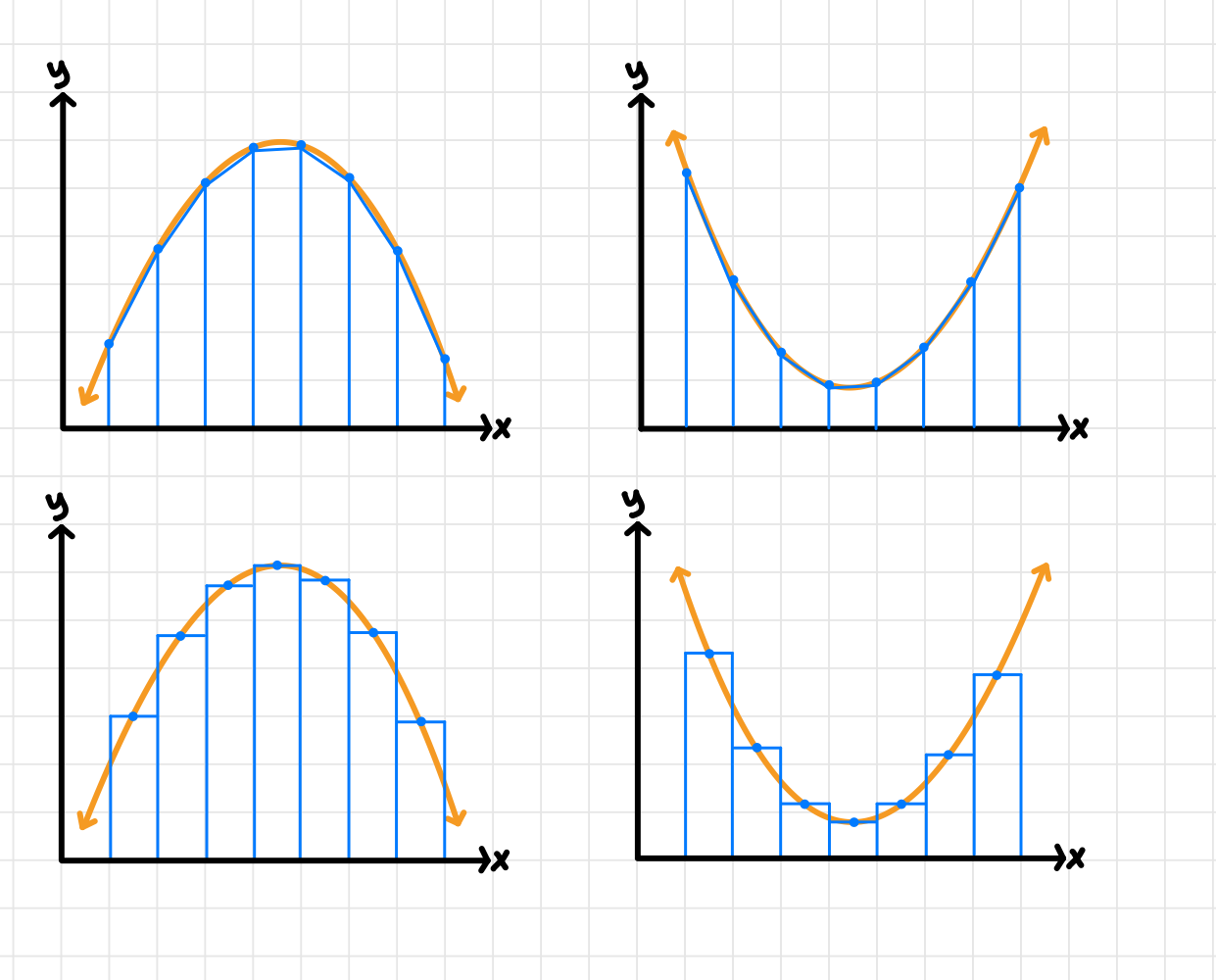
Be familiar with the following:
- A trapezoidal Riemann sum underestimates when a function is concave down.
- A trapezoidal Riemann sum overestimates when a function is concave up.
- A midpoint Riemann sum underestimates when a function is concave up.
- A midpoint Riemann sum overestimates when a function is concave down.
🔢 Numerical Riemann Sums
Sometimes we’re not given a graph to base our estimates on! Let’s work through a sample problem to learn how to approach these types of problems.
Given the function , find , and over the interval [0,4].
The very first thing you should do in this type of problem is draw a graph!
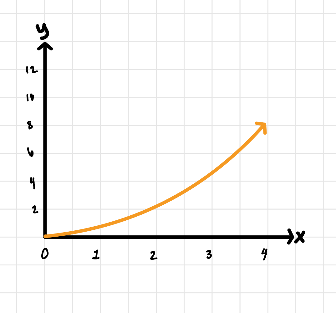
Then, pick one of the Riemann sums to calculate. We’re going to solve for and first.
First, figure out how wide each rectangle will be by dividing the total interval by the number of subdivisions we want:
Then, draw our rectangles on the graph for each type of endpoint:
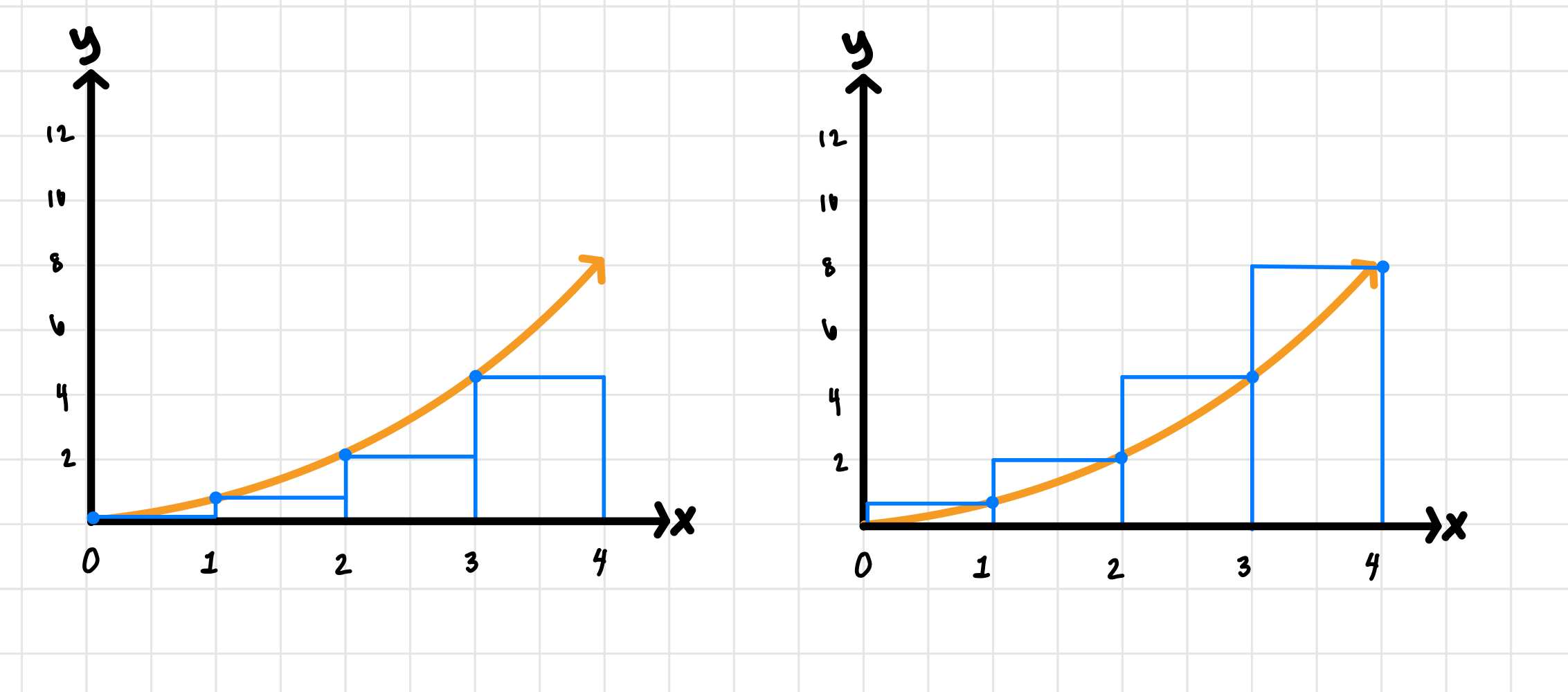
We can also make a table of values from the graph:
| x | y (height) |
|---|---|
| 0 | 0 |
| 1 | 0.5 |
| 2 | 2 |
| 3 | 4.5 |
| 4 | 8 |
Based on our graphs, to find we need to use the left endpoints, which are . Since our base width is 1, we can just sum their values. Thus,
Let’s do the same thing for , using :
Now on to !
We know that there will be four trapezoids since we are using the same number of subdivisions. We can draw it like this:
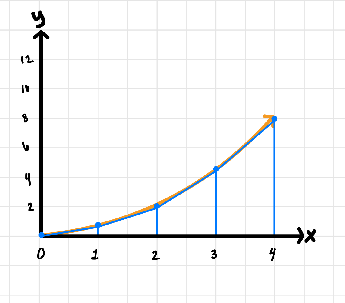
We can also use the same table of values from the first part of the problem to find our values for and .
| x | y (height) |
|---|---|
| 0 | 0 |
| 1 | 0.5 |
| 2 | 2 |
| 3 | 4.5 |
| 4 | 8 |
Let’s plug these values into our equation to find the area of our first trapezoid:
We can do this for all four trapezoids and add them up to get our total area:
Finally, let’s find , starting by drawing our rectangles onto the graph:
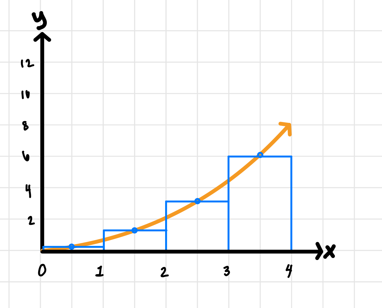
First, we can plug in our x-values from the graph to find the height of each rectangle:
| x | y (height) |
|---|---|
| 0.5 | 0.125 |
| 1.5 | 1.125 |
| 2.5 | 3.125 |
| 3.5 | 6.125 |
Since our the width of each base is just 1, we can simply sum the four values to get our area under the curve estimated by :
Bonus Question: Are and overestimates or underestimates?
Solution: is an overestimate and is an underestimate, which means the true area under the curve lies somewhere between 10.5 and 11!
📝 Practice Problems and Solutions
Now take some time to practice these on your own!
❓Questions
- Given the function over the interval , calculate the Riemann sum with using the right endpoints of each subinterval.
- A function is defined over the interval . Compute the left Riemann sum with for this function.
- Given the function over the interval , find and .
✏️ Solutions
Problem 1 Solution:
First, let’s graph this function over the given interval:
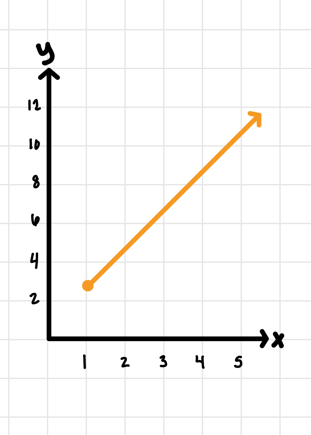
Then, let’s figure out what the width of our rectangles will be and graph with the right endpoints: .
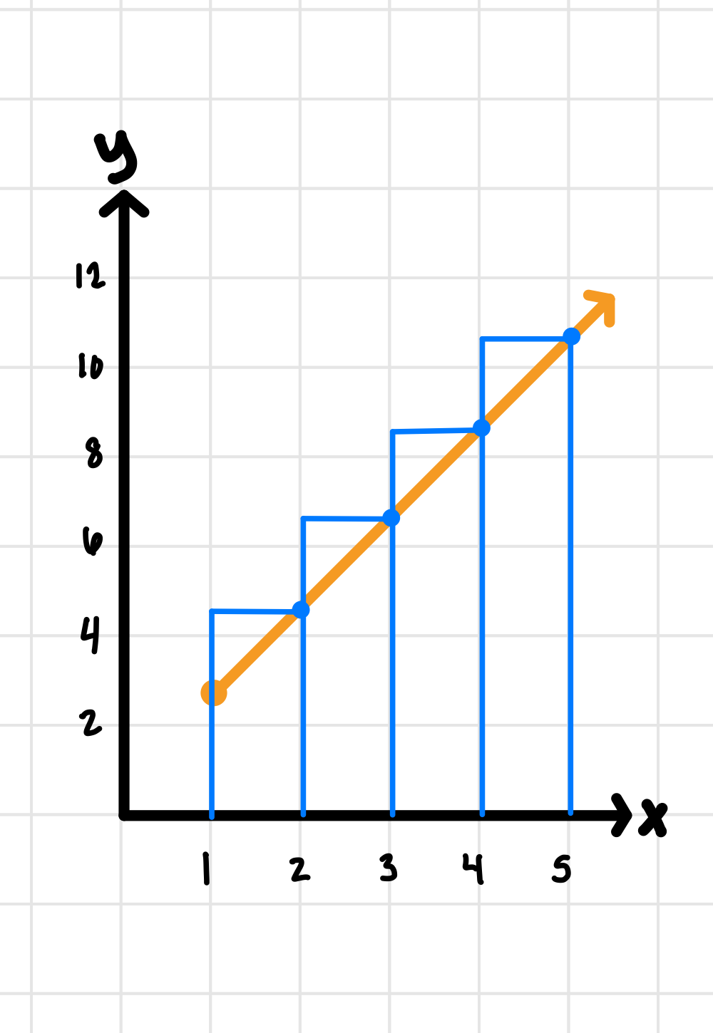
Now, let’s find their heights numerically:
| x-value | y (height) |
|---|---|
| 2 | 5 |
| 3 | 7 |
| 4 | 9 |
| 5 | 11 |
Now, let’s solve by summing the areas of each rectangle:
Problem 2 Solution:
First, let’s graph this function over the given interval:
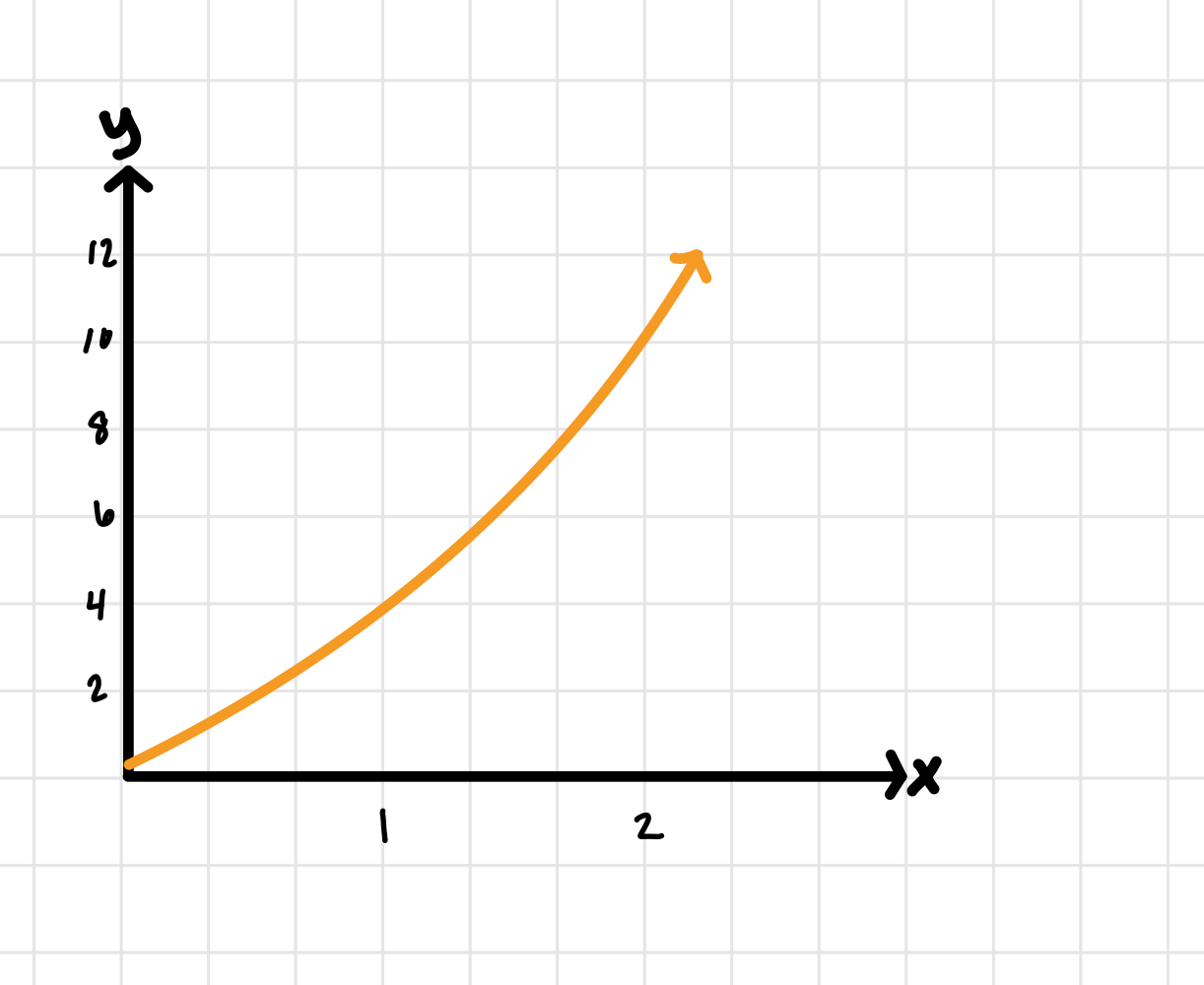
Then, let’s figure out the width of our rectangles and graph with the left endpoints:

Now, let’s find their heights numerically:
| x-value | y (height) |
|---|---|
| 0 | 0 |
| 1/3 | 10/9 |
| 2/3 | 22/9 |
| 1 | 4 |
| 4/3 | 52/9 |
| 5/3 | 70/9 |
Now, let’s solve by summing the areas of each rectangle:
We can rewrite this by factoring out our base length like so:
Problem 3 Solution:
First, let’s graph the function over the given interval:

Then, let’s figure out the width of our rectangles and graph with the trapezoids:

Let’s start by solving for by creating a table of values:
| x-value | y (height) |
|---|---|
| 2 | 8 |
| 2.5 | 14.75 |
| 3 | 23 |
| 3.5 | 32.75 |
| 4 | 44 |
| 4.5 | 56.75 |
| 5 | 71 |
| 5.5 | 86.75 |
| 6 | 104 |
| 6.5 | 122.75 |
| 7 | 143 |
| 7.5 | 164.75 |
| 8 | 188 |
Now, let’s plug it into our equation:
And simplify!
Let’s do the same with midpoints:
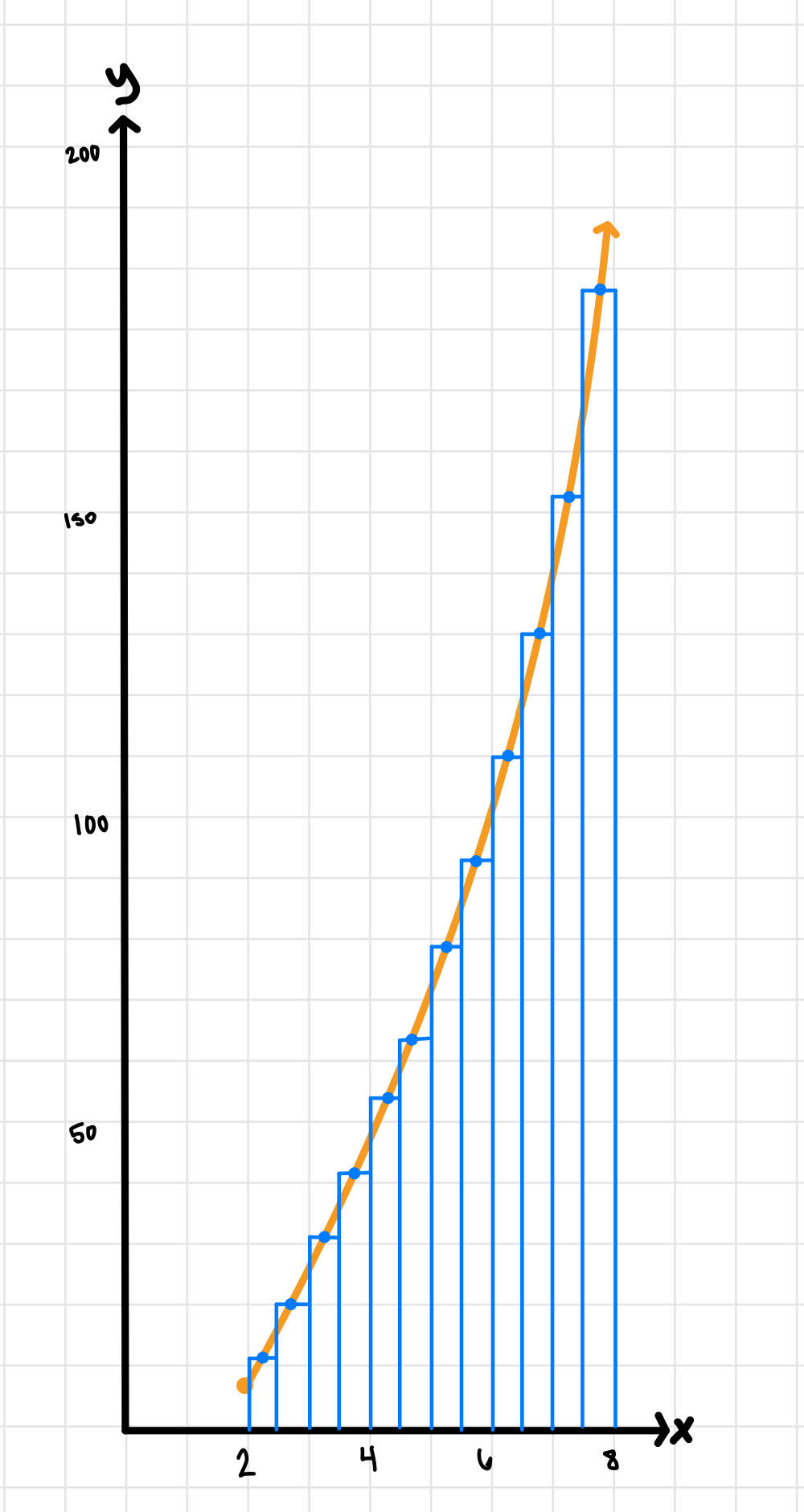
| x-value | y (height) |
|---|---|
| 2.25 | 11.1875 |
| 2.75 | 18.6875 |
| 3.25 | 27.6875 |
| 3.75 | 38.1875 |
| 4.25 | 50.1875 |
| 4.75 | 63.6875 |
| 5.25 | 78.6875 |
| 5.75 | 95.1875 |
| 6.25 | 113.1875 |
| 6.75 | 132.6875 |
| 7.25 | 153.6875 |
| 7.75 | 176.1875 |
Now, let’s plug in and solve:
🌟 Closing
Here are the key takeaways you should now understand about Riemann sums:
- What a left, right, trapezoidal, or midpoint Riemann sum is and…
- How to calculate their values numerically
- When they are overestimates or underestimates
- How to determine the width of rectangles or trapezoids
- How to depict Riemann sums graphically
Best of luck! 🍀
Vocabulary
The following words are mentioned explicitly in the College Board Course and Exam Description for this topic.Term | Definition |
|---|---|
definite integral | The integral of a function over a specific interval [a, b], representing the net signed area between the curve and the x-axis. |
left Riemann sum | An approximation method for a definite integral using rectangles whose heights are determined by the function values at the left endpoints of subintervals. |
midpoint Riemann sum | An approximation method for a definite integral using rectangles whose heights are determined by the function values at the midpoints of subintervals. |
nonuniform partition | A division of an interval into subintervals of varying widths. |
numerical methods | Computational techniques used to approximate definite integrals when exact analytical solutions are difficult or impossible to obtain. |
overestimate | An approximation that is greater than the actual value of a function. |
right Riemann sum | An approximation method for a definite integral using rectangles whose heights are determined by the function values at the right endpoints of subintervals. |
trapezoidal sum | An approximation method for a definite integral using trapezoids to estimate the area under a curve. |
underestimate | An approximation that is less than the actual value of a function. |
uniform partition | A division of an interval into subintervals of equal width. |
Frequently Asked Questions
How do I calculate a left Riemann sum step by step?
A left Riemann sum approximates ∫_a^b f(x) dx by adding up rectangles whose heights are the function values at the left endpoints of subintervals. Step-by-step: 1. Partition [a,b] into n subintervals. For a uniform partition, Δx = (b−a)/n. 2. Label points: x0 = a, x1 = a+Δx, …, xn = b. 3. Choose left endpoints as your sample points: for the i-th rectangle use xi−1 (i = 1..n). 4. Compute each rectangle area: f(xi−1)·Δx. 5. Sum them: Left sum L_n = Σ_{i=1}^n f(x_{i−1}) Δx. 6. Evaluate numerically (or let technology do it for large n). Quick check for AP-style reasoning (CED LIM-5.A.2/LIM-5.A.4): if f is decreasing on [a,b], the left sum is an overestimate; if f is increasing, it’s an underestimate. For nonuniform partitions use Δx_i and xi−1 for each term: Σ f(x_{i−1}) Δx_i. For a practice walkthrough and examples, see the Topic 6.2 study guide (https://library.fiveable.me/ap-calculus/unit-6/approximating-areas-with-riemann-sums/study-guide/juN9YbvFYlJtpsMl). For more problems, try Fiveable’s AP practice set (https://library.fiveable.me/practice/ap-calculus).
What's the difference between left, right, and midpoint Riemann sums?
Left, right and midpoint Riemann sums are just three ways to pick a sample point in each subinterval when you approximate a definite integral ∫_a^b f(x) dx. - Partition the interval into subintervals of widths Δx (uniform or nonuniform). - Left Riemann sum: use the left endpoint of each subinterval. Sum = Σ f(x_k_left)·Δx. - Right Riemann sum: use the right endpoint. Sum = Σ f(x_k_right)·Δx. - Midpoint Riemann sum: use the midpoint of each subinterval. Sum = Σ f(x_k_mid)·Δx. Which is better depends on the function: if f is increasing, left sums underestimate and right sums overestimate (reverse if f is decreasing). Midpoint sums usually give a more accurate approximation for smooth functions because positive and negative errors cancel more; the midpoint error is O(Δx^2) for nice f (same order as trapezoid but often smaller constant). On the AP exam you should be comfortable computing these with uniform or nonuniform partitions, writing them in summation notation, and using monotonicity/concavity to state over/underestimate (CED LIM-5.A and LIM-5.A.2). For a quick review, see the Topic 6.2 study guide (https://library.fiveable.me/ap-calculus/unit-6/approximating-areas-with-riemann-sums/study-guide/juN9YbvFYlJtpsMl) and try practice problems (https://library.fiveable.me/practice/ap-calculus).
When do I use trapezoidal rule vs midpoint rule for approximating integrals?
Use the midpoint rule when you can sample (or are given) function values at subinterval midpoints and want better accuracy for the same number of subintervals; use the trapezoidal rule when you only (or more easily) have endpoint values or when you want a simple average-of-endpoint-rectangles picture. Key AP rules (CED LIM-5.A keywords: overestimate/underestimate, concavity): - If f''(x) > 0 (concave up) on an interval: trapezoidal rule overestimates the integral (chords lie above the curve); midpoint rule underestimates it. - If f''(x) < 0 (concave down): trapezoid underestimates and midpoint overestimates. So you can decide which to trust by checking concavity on the interval (or graph/table). Accuracy note (useful on the exam): for a uniform partition of n subintervals, the error magnitudes satisfy - Trapezoid error ≈ -(b−a)^3/(12 n^2) · f''(ξ) - Midpoint error ≈ -(b−a)^3/(24 n^2) · f''(η) So midpoint typically has about half the error of trapezoid (same n). For more practice and AP-style problems see the Topic 6.2 study guide (https://library.fiveable.me/ap-calculus/unit-6/approximating-areas-with-riemann-sums/study-guide/juN9YbvFYlJtpsMl) and lots of problems at (https://library.fiveable.me/practice/ap-calculus).
I'm confused about how to set up the formula for right Riemann sums - can someone explain?
For a right Riemann sum on [a,b], first pick a partition of n subintervals (uniform is usual on the AP). Then - Δx = (b − a)/n. - Right endpoints: x_k = a + k·Δx for k = 1, 2, …, n. - Right Riemann sum: R_n = Σ_{k=1}^n f(x_k)·Δx. So you evaluate f at the right endpoint of each subinterval, multiply each value by the subinterval width, and add. In limit form (definite integral): ∫_a^b f(x) dx = lim_{n→∞} Σ_{k=1}^n f(a + kΔx)·Δx when the limit exists (CED LIM-5.A). Quick tips: for nonuniform partitions use each actual Δx_k and right sample x_k* (R = Σ f(x_k*)Δx_k). If f is increasing on [a,b], the right sum overestimates; if f is decreasing, it underestimates (use monotonicity to judge error). For more examples and AP-style practice, see the Topic 6.2 study guide (https://library.fiveable.me/ap-calculus/unit-6/approximating-areas-with-riemann-sums/study-guide/juN9YbvFYlJtpsMl), the Unit 6 overview (https://library.fiveable.me/ap-calculus/unit-6), and extra practice problems (https://library.fiveable.me/practice/ap-calculus).
How do I know if my Riemann sum approximation is an overestimate or underestimate?
Quick test: look at f' (increasing/decreasing) and f'' (concavity). - Monotonic rule (left/right sums, uniform partition): - If f is increasing on [a,b]: left Riemann sum underestimates, right Riemann sum overestimates. - If f is decreasing: left overestimates, right underestimates. Reason: sample heights come from the lower or upper end of each subinterval. - Concavity rule (midpoint and trapezoid): - If f is concave up (f''>0): trapezoidal rule overestimates and midpoint rule underestimates. - If f is concave down (f''<0): trapezoid underestimates and midpoint overestimates. Reason: trapezoids connect endpoints (sit above the curve when concave up); midpoints use central height (sit below when concave up). Notes: For nonuniform partitions, decide per-subinterval using local monotonicity/concavity. If you don’t have derivatives, use the graph. On the AP exam you’ll be asked to justify with f' or f'' signs or by comparing rectangle/trapezoid placement. For more review see the Topic 6.2 study guide (https://library.fiveable.me/ap-calculus/unit-6/approximating-areas-with-riemann-sums/study-guide/juN9YbvFYlJtpsMl) and tons of practice problems (https://library.fiveable.me/practice/ap-calculus).
What's the formula for calculating delta x when finding Riemann sums?
For a uniform partition of [a, b], Δx = (b − a)/n (where n is the number of subintervals). Then a Riemann sum looks like Σ_{k=1}^n f(x_k*)·Δx, where x_k* is a sample point in the k-th subinterval (left, right, midpoint, or any sample). If the partition is nonuniform, you don’t use a single Δx—each subinterval has its own width Δx_k = x_k − x_{k−1}, and the sum is Σ f(x_k*)·Δx_k. This matches the AP Topic 6.2 ideas: use uniform or nonuniform partitions and choose left/right/midpoint samples to get approximations (see the Topic 6.2 study guide for examples) (https://library.fiveable.me/ap-calculus/unit-6/approximating-areas-with-riemann-sums/study-guide/juN9YbvFYlJtpsMl). For exam problems expect Δx = (b−a)/n when they say “n equal subintervals.”
Can someone walk me through how to approximate a definite integral using left endpoints?
Use a partition of [a,b] into n subintervals (uniform for AP problems unless told otherwise). Steps: 1. Compute Δx = (b − a)/n. 2. For left endpoints use x_k = a + k·Δx for k = 0,1,...,n−1. 3. Form the left Riemann sum L_n = Σ_{k=0}^{n−1} f(x_k)·Δx. This approximates ∫_a^b f(x) dx. 4. Interpret error by monotonicity: if f is increasing on [a,b], L_n is an underestimate; if f is decreasing, L_n is an overestimate (CED LIM-5.A.2/LIM-5.A.4). Quick example: approximate ∫_1^3 f(x) dx with n=4. Δx=(3−1)/4=0.5. Left x_k = 1.0,1.5,2.0,2.5. Then L_4 = 0.5[f(1)+f(1.5)+f(2)+f(2.5)]. Left sums fit AP tasks: you may be asked to set up a sum, evaluate numerically, or state under/overestimate reasoning. For extra review, see the Topic 6.2 study guide (https://library.fiveable.me/ap-calculus/unit-6/approximating-areas-with-riemann-sums/study-guide/juN9YbvFYlJtpsMl), Unit 6 overview (https://library.fiveable.me/ap-calculus/unit-6) and lots of practice problems (https://library.fiveable.me/practice/ap-calculus).
I don't understand how to determine the number of rectangles to use in a Riemann sum problem.
You don’t pick n arbitrarily—the problem tells you how many rectangles or how the partition is set. Here’s how to decide: - If the problem gives n, use it. For a uniform partition Δx = (b − a)/n and sample points xk (left, right, midpoint) to build Σ f(xk)Δx. - If it gives subinterval endpoints (nonuniform), use those widths Δxk shown. - If it asks for a limit as n → ∞, write the Riemann sum with Δx = (b − a)/n and convert to the integral (limit form). - If it asks for an approximation without specifying n, choose n large enough for desired accuracy (bigger n → better approximation). Use midpoint or trapezoid for better accuracy with fewer rectangles. - Use function behavior to judge error: if f is increasing, left sums underestimate and right sums overestimate; concavity tells you whether trapezoid over/underestimates (CED LIM-5.A.4). Want practice picking n and estimating errors? Check the Topic 6.2 study guide (https://library.fiveable.me/ap-calculus/unit-6/approximating-areas-with-riemann-sums/study-guide/juN9YbvFYlJtpsMl) and try problems on Fiveable’s practice page (https://library.fiveable.me/practice/ap-calculus).
How do I use my calculator to find Riemann sum approximations?
Yes—you can use your graphing calculator to get Riemann-sum approximations quickly. Here’s a short, AP-aligned how-to (works on TI-83/84 family and similar calculators): 1. Pick interval [a,b], n subintervals, Δx = (b−a)/n. Decide left/right/mid sample points: - Left: x_k = a + (k−1)Δx - Right: x_k = a + kΔx - Mid: x_k = a + (k−0.5)Δx 2. Use the calculator’s sum and seq commands (TI syntax shown): - Left Riemann: sum(seq(f(a+(k-1)*Δx), k, 1, n))*Δx - Right Riemann: sum(seq(f(a+k*Δx), k, 1, n))*Δx - Midpoint: sum(seq(f(a+(k-0.5)*Δx), k, 1, n))*Δx Example (TI-84): Δx→dx; sum(seq( yourFunction(a+(k-1)*dx), k,1,n))*dx 3. If your calculator supports lists: create list Xk with sample points, create list F = f(Xk), then ΣF * Δx. 4. For trapezoidal rule use: (Δx/2)*(f(a)+2Σf(interiors)+f(b))—you can implement with seq or lists. Remember: calculators are allowed on Part B (last 15 MC) and Part A of Section II (2 FR Qs) on the AP exam, so practice these commands under timed conditions. For more step-by-step examples and AP-style practice, see the Topic 6.2 study guide (https://library.fiveable.me/ap-calculus/unit-6/approximating-areas-with-riemann-sums/study-guide/juN9YbvFYlJtpsMl) and the unit page (https://library.fiveable.me/ap-calculus/unit-6). For extra practice problems, try (https://library.fiveable.me/practice/ap-calculus).
What does it mean when a problem asks for a "uniform partition" in Riemann sums?
A "uniform partition" means you split the interval [a, b] into n subintervals all the same width. So Δx = (b − a)/n and the partition points are a, a+Δx, a+2Δx, …, b. For Riemann sums you then pick a sample point in each equal subinterval (left, right, or midpoint) and form Σ f(sample_k)·Δx. Why it matters: uniform partitions make the algebra and limits cleaner (e.g., turning sums into closed-form expressions and taking n → ∞ to get the definite integral). The CED calls out both uniform and nonuniform partitions (LIM-5.A.2); if a problem says “uniform,” don’t use variable-width Δx_k—use the single Δx above. Also remember the norm (mesh) of the partition is max subinterval width; for uniform partitions the norm = Δx. For quick practice and AP-style problems see the Topic 6.2 study guide (https://library.fiveable.me/ap-calculus/unit-6/approximating-areas-with-riemann-sums/study-guide/juN9YbvFYlJtpsMl) and the practice problem bank (https://library.fiveable.me/practice/ap-calculus).
Why does the midpoint rule usually give better approximations than left or right Riemann sums?
The midpoint rule usually gives better approximations because it samples each subinterval at its center, which tends to cancel positive and negative errors from the subintervals—and mathematically its error decreases faster. For a smooth function (f twice differentiable) on a uniform partition, the midpoint error on [a,b] is proportional to f''(ξ)·(b−a)^3/(24n^2), while left/right Riemann sums generally have errors that shrink only like 1/n when the function is monotone (and their sign depends on monotonicity). So midpoint is often O(1/n^2) accuracy versus O(1/n) for left/right, and its error constant is smaller than trapezoid’s as well. Use monotonicity/concavity (CED LIM-5.A.4) to tell whether left/right are over- or underestimates; use midpoint when you can assume smoothness for better accuracy. For review and practice, see the Topic 6.2 study guide (https://library.fiveable.me/ap-calculus/unit-6/approximating-areas-with-riemann-sums/study-guide/juN9YbvFYlJtpsMl) and more problems at the Unit 6 page (https://library.fiveable.me/ap-calculus/unit-6) or practice set (https://library.fiveable.me/practice/ap-calculus).
How do I solve Riemann sum problems when the function is given as a table of values instead of an equation?
When the function is given in a table, you do the same Riemann-sum idea but use the table values as your sample points. Steps: 1. Partition & Δx: use the x-values in the table. If they’re equally spaced, Δx is that spacing; if not, each subinterval has its own Δx (nonuniform partition). 2. Pick sample points: for a left Riemann sum use the left endpoint value from the table for each subinterval; for right use the right endpoint; for midpoint use a table value at the midpoint (if given). For trapezoidal, average the two endpoint values for each subinterval. 3. Compute: sum f(xi*)·Δx_i across subintervals. Example (uniform 1-unit intervals, left sum): Σ f(x_k)·1. 4. Error direction: use LIM-5.A.4—if f is increasing a left sum underestimates and a right sum overestimates; check concavity for trapezoid/midpoint behavior. This matches AP expectations (CED LIM-5.A: numeric/tabular approximations). For more examples and practice, see the Topic 6.2 study guide (https://library.fiveable.me/ap-calculus/unit-6/approximating-areas-with-riemann-sums/study-guide/juN9YbvFYlJtpsMl), the Unit 6 overview (https://library.fiveable.me/ap-calculus/unit-6), and lots of practice problems (https://library.fiveable.me/practice/ap-calculus).
What's the difference between LRAM, RRAM, MRAM, and TRAP on the AP exam?
LRAM, RRAM, MRAM, and TRAP are just different ways to build Riemann-sum approximations for ∫_a^b f(x) dx using sample points on subintervals: - LRAM (Left): sum f(x_{k-1}) Δx. Use left endpoint heights. - RRAM (Right): sum f(x_k) Δx. Use right endpoint heights. - MRAM (Midpoint): sum f((x_{k-1}+x_k)/2) Δx. Use midpoint heights—usually more accurate (error ~ 1/n^2). - TRAP (Trapezoidal): sum [f(x_{k-1})+f(x_k)]/2 · Δx. Uses trapezoids, blends left and right. On the AP: you should know formulas for uniform or nonuniform partitions and be able to tell over/underestimate using monotonicity and concavity (CED LIM-5.A.2 & LIM-5.A.4). Quick rules: if f is increasing on an interval, LRAM underestimates and RRAM overestimates (reverse if decreasing). For concavity: if f is concave up, trapezoidal rule overestimates and midpoint underestimates (opposite when concave down). Practice these on the Topic 6.2 study guide (https://library.fiveable.me/ap-calculus/unit-6/approximating-areas-with-riemann-sums/study-guide/juN9YbvFYlJtpsMl) and drill problems at (https://library.fiveable.me/practice/ap-calculus).
I keep getting confused about whether to use f(xi) or f(xi-1) in my Riemann sum formula - which is correct?
Use whichever sample point the problem (or your choice of Riemann sum) tells you—there isn’t a single “correct” one. The general Riemann sum is sum_{k=1}^n f(x_k^*) Δx, where x_k^* is the sample point in the k-th subinterval. Common choices: - Left Riemann sum: x_k^* = x_{k-1} so sum = Σ f(x_{k-1}) Δx. - Right Riemann sum: x_k^* = x_k so sum = Σ f(x_k) Δx. - Midpoint: x_k^* = (x_{k-1}+x_k)/2 so sum = Σ f(midpoint) Δx. If the problem asks for a left (or right, midpoint) sum, use the corresponding sample point. If it gives a partition indexed 0..n, be careful: “left” uses f(x_{k-1}) for k=1..n; “right” uses f(x_k). Which one is an over/underestimate depends on monotonicity (increasing f: left underestimates, right overestimates) and concavity matters for trapezoid/midpoint error—exactly the ideas in the AP CED (LIM-5.A, LIM-5.A.2, LIM-5.A.4). For a quick refresher and examples, see the Topic 6.2 study guide (https://library.fiveable.me/ap-calculus/unit-6/approximating-areas-with-riemann-sums/study-guide/juN9YbvFYlJtpsMl). For more practice problems, go to (https://library.fiveable.me/practice/ap-calculus).
How do I approximate the area under a curve when the intervals aren't all the same width?
If the subintervals aren’t equal, you still form a Riemann sum—just use each subinterval’s actual width. For a partition a = x0 < x1 < ... < xn = b, pick a sample point xk* in [xk-1, xk] and compute sum_{k=1}^n f(xk*) Δx_k , where Δx_k = x_k − x_{k-1}. That single formula covers left/right/midpoint choices (choose xk* = xk-1, xk, or (xk-1+xk)/2). The trapezoidal sum also works with nonuniform Δx_k by adding ½[f(xk-1)+f(xk)]Δx_k for each subinterval. As the norm (largest Δx_k) → 0 the Riemann sums converge to the definite integral ∫_a^b f(x) dx (CED LIM-5.A.2). Use monotonicity/concavity to judge over/underestimates: e.g., if f is increasing on [xk-1,xk], left-sum on that subinterval underestimates and right-sum overestimates. For practice and AP-style examples see the Topic 6.2 study guide (https://library.fiveable.me/ap-calculus/unit-6/approximating-areas-with-riemann-sums/study-guide/juN9YbvFYlJtpsMl) and try extra problems at (https://library.fiveable.me/practice/ap-calculus).