Confidence Intervals
As previously stated, there are two kinds of inference: prediction and testing claims. The first type of inference in regards to linear regression we are going to tackle is the prediction model (in other words, confidence intervals).
Confidence intervals are a way to estimate the value of a population parameter based on sample data. They provide a range of values that is likely to contain the true population parameter with a certain level of confidence. For example, if we construct a 95% confidence interval for a population mean, we can be 95% confident that the true population mean lies within the interval. Confidence intervals are useful for making predictions about future samples or for comparing the results of different studies.
The width of the confidence interval depends on the sample size, the level of confidence, and the degree of variation in the sample. A larger sample size, a higher confidence level, and less variation in the sample will result in a narrower confidence interval.
To construct a confidence interval for a population mean, we first need to calculate the standard error of the mean (SEM). The SEM is a measure of the variability of the sample mean. It is calculated as the standard deviation of the sample divided by the square root of the sample size. The SEM gives us an idea of how much the sample mean is likely to vary from the true population mean.
To construct the confidence interval, we then add and subtract a multiple of the SEM from the sample mean. The multiple is chosen based on the desired confidence level. For example, to construct a 95% confidence interval, we would use a multiple of 1.96. So the confidence interval would be the sample mean plus or minus 1.96 times the SEM.
For example, suppose we have a sample of 10 observations with a mean of 10 and a standard deviation of 2. The SEM would be 2/sqrt(10) = 0.6. To construct a 95% confidence interval, we would add and subtract 1.96 times the SEM from the sample mean, resulting in a confidence interval of (8.8, 11.2). This means that we can be 95% confident that the true population mean lies within the interval (8.8, 11.2).
How does this change in the context of this unit (i.e., lines and slopes)?
In linear regression, our biggest interest is the slope of our regression line. While we can somewhat easily calculate the slope of our sample, we know that this slope is going to change as we add more data points and could change greatly if we were to add several more data points; do instead of just relying on our sample slope, it's a much more robust process to construct a confidence interval to find all possible values of our slope!

Point Estimate
The first part of our confidence interval is our point estimate. This is the exact slope of our sample data that can be calculated using the methods discussed in Unit 2. This is the middle of our confidence interval and our starting point. From there, we are going to add and subtract our margin of error to give us a “buffer zone” around our sample prediction.
Margin of Error
Our margin of error for our confidence interval is calculated by using the appropriate t score and the standard deviation of the residuals and standard deviation of the x values.
Our t score is based on the confidence level and degrees of freedom as mentioned in Unit 7.
Our standard error can be calculated using the formula on the formula sheet (below).
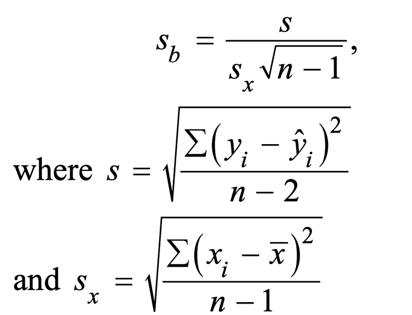
(Note: This formula uses n–2 in the denominator instead of n–1 because two parameters, α and β, must be estimated to obtain the predicted values from the least-squares regression line.)
This formula is very cumbersome and I would always recommend using your graphing calculator to calculate your interval by selecting LinRegTInt and using your L1 and L2 for your sample data.
Side Note: Standard Deviation and Residuals
In linear regression, the sample regression line is an estimate of the population regression line, which represents the underlying relationship between the response variable and the predictor variable in the population. The residuals from the sample regression line are the differences between the observed response values and the predicted response values based on the sample regression line. These residuals can be used to estimate the deviation of the response values from the population regression line.
The standard deviation of the residuals, denoted as s, is a measure of the dispersion of the residuals around the mean. It is calculated as the square root of the sum of the squared residuals divided by n - 2, where n is the sample size. The standard deviation of the residuals can be used to estimate the standard deviation of the deviations of the response values from the population regression line, denoted as σ.
The standard deviation of the residuals is also known as the standard error of the estimate, and it is used to construct confidence intervals and hypothesis tests for the population slope and the population intercept. It can be used to evaluate the fit of the sample regression line and to compare the fits of different regression models.
Conditions
Now, we established that the appropriate confidence interval for the population slope in linear regression is a t-interval, which is based on the t-distribution. Recall from previous units that the t-distribution is a type of probability distribution that is used to estimate population parameters when the sample size is small or when the population standard deviation is unknown.
As with every inference procedure we have covered, there are conditions for inference that must be met if we carry out a test or construct an interval:
(1) Linear
The first and easiest condition to check is that the true relationship between our x and y variable appear to be linear. This can be confirmed by observing the residual plot and seeing that there is no real pattern in the residuals.
(2) Standard Deviation of y
The next condition that must be met is that the standard deviation of y must not change as x changes. In other words, our residual plot does not scatter more or less as we move down the x axis. Again, there is absolutely no pattern on the residual plot
(3) Independence
Independence can be checked two ways:
- Data was taken from a random sample or randomized experiment
- 10% condition (same as other inference procedures): “It is reasonable to believe there is at least 10n… in our population”
(4) Normal
As we have all figured out by now, everything hinges on the normal distribution in statistics. To show normal distribution for quantitative data, we use the Central Limit Theorem, which states that our sample size is at least 30 (or our y values are approximately normal as is).
Once you have checked your conditions, you are good to go in using your sample data to construct and interpret a confidence interval for quantitative means (which I strongly recommend using some form of technology like a graphing calculator to do! Woo-hoo!
Vocabulary
The following words are mentioned explicitly in the College Board Course and Exam Description for this topic.
| Term | Definition |
|---|---|
| confidence interval | A range of values, calculated from sample data, that is likely to contain the true population parameter with a specified level of confidence. |
| critical value | A value from the standard normal distribution used to determine the margin of error for a given confidence level. |
| explanatory variable | A variable whose values are used to explain or predict corresponding values for the response variable. |
| independence | The condition that observations in a sample are not influenced by each other, typically ensured through random sampling or randomized experiments. |
| least-squares regression line | A linear model that minimizes the sum of squared residuals to find the best-fitting line through a set of data points. |
| linearity | The condition that the true relationship between two variables follows a straight line. |
| margin of error | The amount by which a sample statistic is likely to vary from the corresponding population parameter, calculated as the critical value times the standard error. |
| normality | The condition that data follows an approximately normal (bell-shaped) distribution. |
| population regression line | The true linear relationship μy = α + βx between the response and explanatory variables in the entire population. |
| random sample | A sample selected from a population in such a way that every member has an equal chance of being chosen, reducing bias and allowing for valid statistical inference. |
| randomized experiment | A study design where subjects are randomly assigned to treatment groups to establish cause-and-effect relationships. |
| regression model | A statistical model that describes the relationship between a response variable (y) and one or more explanatory variables (x). |
| residual | The difference between the actual observed value and the predicted value in a regression model, calculated as residual = y - ŷ. |
| response variable | A variable whose values are being explained or predicted based on the explanatory variable. |
| sample regression line | The line ŷ = a + bx calculated from sample data that estimates the population regression line. |
| sample statistic | A numerical value calculated from sample data that is used to estimate the corresponding population parameter. |
| sampling distribution | The probability distribution of a sample statistic (such as a sample proportion) obtained from repeated sampling of a population. |
| sampling without replacement | A sampling method in which an item selected from a population cannot be selected again in subsequent draws. |
| simple random sample | A sample selected from a population such that every possible sample of the same size has an equal chance of being chosen. |
| skewed | A distribution that is not symmetric, with one tail longer or more pronounced than the other. |
| slope | The value b in the regression equation ŷ = a + bx, representing the rate of change in the predicted response for each unit increase in the explanatory variable. |
| slope of a regression model | The coefficient that represents the rate of change in the predicted response variable for each unit increase in the explanatory variable in a linear regression equation. |
| standard deviation | A measure of how spread out data values are from the mean, represented by σ in the context of a population. |
| standard deviation of residuals | A measure of the spread of residuals around the regression line, estimated by s = √(Σ(yi - ŷi)²/(n-2)). |
| standard deviation of x values | A measure of the spread of the x-variable values in the sample, denoted as sx in the standard error formula. |
| standard error of the slope | A measure of the variability of the slope estimate across different samples, calculated as s divided by (sx times the square root of n-1). |
| t-interval | A confidence interval procedure that uses the t-distribution, appropriate for estimating the slope of a regression model. |
| t* | The critical value from the t-distribution used to construct a confidence interval for the slope of a regression model. |
Frequently Asked Questions
How do I find the confidence interval for the slope of a regression line?
You use a t-interval around the sample slope b: b ± t*·SEb. Steps: 1. Verify conditions (linearity, constant spread, independence, near-normal residuals; df = n−2). Use residual plots to check linearity/heteroscedasticity as the CED requires. 2. Compute s = √[Σ(yi−ŷi)²/(n−2)] and sx = sample SD of x. 3. Standard error of the slope: SEb = s / (sx·√(n−1)) (CED formula). 4. Choose confidence level and get t* with df = n−2 (from the t-table or calculator). 5. Margin of error = t*·SEb. Confidence interval = b ± t*·SEb. Interpretation: the interval gives plausible values for the population slope β. If 0 is not in the interval, there’s evidence of a linear relationship. For more practice and AP-aligned examples, see the Topic 9.2 study guide (https://library.fiveable.me/ap-statistics/unit-9/confidence-intervals-for-slope-regression-model/study-guide/YsvXWrndemJrI2kBF3Wn) and unit review (https://library.fiveable.me/ap-statistics/unit-9). For lots of practice problems go to (https://library.fiveable.me/practice/ap-statistics).
What's the formula for the standard error of the slope in regression?
The standard error of the slope (SEb) you use in a t-interval for the slope is SEb = s / (sx · √(n − 1)), where s = √[Σ(yi − ŷi)²/(n − 2)] is the sample estimate of the residual standard deviation, sx = √[Σ(xi − x̄)²/(n − 1)] is the sample standard deviation of x, and n is the sample size. The CI for the population slope β is b ± t* · SEb with df = n − 2. This matches the AP CED formula and the margin-of-error idea: margin = t*·SE. For a quick review, see the Topic 9.2 study guide (https://library.fiveable.me/ap-statistics/unit-9/confidence-intervals-for-slope-regression-model/study-guide/YsvXWrndemJrI2kBF3Wn) and the Unit 9 overview (https://library.fiveable.me/ap-statistics/unit-9). For extra practice, check the AP Stats practice problems (https://library.fiveable.me/practice/ap-statistics).
When do I use a t-interval vs z-interval for regression slope confidence intervals?
Use a t-interval. For slope inference you almost always use t because the population error standard deviation σ is unknown and you estimate it with s (the SD of residuals). The sampling distribution of the sample slope b is centered at β and its SE uses s and sx, and the CI is b ± t*·SEb with t* from a t-distribution with df = n − 2 (CED: UNC-4.AC, UNC-4.AF). Quick checklist: verify linearity, constant σ (homoscedasticity), independence (random sample or experiment; n ≤ 10% N if no replacement), and roughly normal residuals (use plots; if skewed need n > 30)—those are the AP conditions (UNC-4.AD). On the exam use t* from the table or your calculator; AP supplies t tables (and you’ll use df = n−2). For a refresher see the Topic 9.2 study guide (https://library.fiveable.me/ap-statistics/unit-9/confidence-intervals-for-slope-regression-model/study-guide/YsvXWrndemJrI2kBF3Wn) and more unit practice (https://library.fiveable.me/ap-statistics/unit-9). For extra practice try the AP question bank (https://library.fiveable.me/practice/ap-statistics).
I'm confused about checking conditions for regression slope confidence intervals - what do I need to verify?
You need to check four AP-approved conditions before using a t–confidence interval for the slope (UNC-4.AD): 1. Linearity—the true relationship between x and y is linear. Use a scatterplot and the residual plot: residuals should show no curved pattern. 2. Constant variability (homoscedasticity)—σy doesn’t change with x. In the residual plot, the spread of residuals should be roughly the same for all x. 3. Independence—data come from a random sample or randomized experiment; if sampling without replacement, verify n ≤ 10% of the population. 4. Normality of responses for a given x—residuals (for each x) should be approximately normal. Check a residual histogram or normal probability plot. If residuals are skewed, CED says n should be > 30 to rely on the t-interval. If these look OK, you can compute b ± t*(SEb) with SEb = s/(sx√(n−1)) and df = n−2. For a quick AP review, see the Topic 9.2 study guide (https://library.fiveable.me/ap-statistics/unit-9/confidence-intervals-for-slope-regression-model/study-guide/YsvXWrndemJrI2kBF3Wn)—and try practice problems at (https://library.fiveable.me/practice/ap-statistics).
How do I know if the linear condition is met when looking at residual plots?
Check the residual plot for randomness around the horizontal line y = 0. If the residuals are scattered with no clear pattern and hover roughly equally above and below zero, the linear condition is likely met (this is what the CED means by “analysis of residuals may be used to verify linearity”). Specific things to look for: - No curved pattern (U-shape or systematic curve → relationship not linear). - No trend in residual size across x (if residuals get larger or smaller with x—a funnel shape—that's heteroscedasticity, violating equal σ_y). - No big clusters or long runs of positive/negative residuals (could signal model misspecification or dependence). - Center of residuals ≈ 0 and roughly constant spread for all x. For normality of responses at a given x, check a histogram or normal Q-Q of residuals; if residuals look skewed, the CED recommends n > 30 to rely on approximate normality. Also verify data collection was random (independence). For practice and AP-focused review on checking residuals and conditions for CIs for slope, see the Topic 9.2 study guide (https://library.fiveable.me/ap-statistics/unit-9/confidence-intervals-for-slope-regression-model/study-guide/YsvXWrndemJrI2kBF3Wn) and the Unit 9 overview (https://library.fiveable.me/ap-statistics/unit-9). For more practice problems, use (https://library.fiveable.me/practice/ap-statistics).
What's the difference between the population regression line and sample regression line?
The population regression line is the true, unknown relationship in the whole population: μy = α + βx (α and β are population parameters). The sample regression line is what you calculate from your data: ŷ = a + bx (a and b are estimates). Key differences from the CED: residuals yi − ŷi estimate the population deviations yi − (α + βxi); the sample residual standard deviation s = √[Σ(yi−ŷi)²/(n−2)] estimates the population σ; and the sampling distribution of the sample slope b has mean β (μb = β) and standard error s_b = s / (s_x√(n−1)) (use this SE in the t-interval). So b ± t*·SEb gives a confidence interval for β. Always check linearity, equal variance, independence, and (approx.) normality of residuals before making inference (see Topic 9.2 study guide for details: https://library.fiveable.me/ap-statistics/unit-9/confidence-intervals-for-slope-regression-model/study-guide/YsvXWrndemJrI2kBF3Wn; unit overview: https://library.fiveable.me/ap-statistics/unit-9). For practice, try problems at https://library.fiveable.me/practice/ap-statistics.
Can someone explain step by step how to calculate a confidence interval for regression slope?
Step-by-step (use your calculator or software for sums): 1. Fit the least-squares line and get b (sample slope), residuals, n. 2. Compute s, the SD of residuals: s = sqrt[Σ(yi − ŷi)² / (n − 2)]. 3. Compute sx, the sample SD of x: sx = sqrt[Σ(xi − x̄)² / (n − 1)]. 4. Find the standard error of the slope: SEb = s / (sx · sqrt(n − 1)). (This is the AP CED formula.) 5. Choose your confidence level (e.g., 95%) and get t* with df = n − 2 from Table B (or your calculator). 6. Compute margin of error: ME = t* · SEb. 7. Construct the interval: b ± ME. Interpret in context as a CI for the population slope β. Before using the interval, verify AP conditions: linearity, constant σy (homoscedasticity), independence (random sample or n ≤ 10% N), and approximate normality of residuals (or n > 30 if skewed). For a quick refresher and worked examples see the Fiveable Topic 9.2 study guide (https://library.fiveable.me/ap-statistics/unit-9/confidence-intervals-for-slope-regression-model/study-guide/YsvXWrndemJrI2kBF3Wn) and more practice (https://library.fiveable.me/practice/ap-statistics).
Why does the residual standard deviation formula use n-2 instead of n-1 in the denominator?
Because when you fit a least-squares line you’ve estimated two unknown population parameters (α and β), you lose two degrees of freedom. The residual standard deviation s is trying to estimate the population scatter σ of y around the true regression line. To get unbiased variability you divide the sum of squared residuals by the number of independent pieces of information left after estimating parameters—that's n − 2, not n − 1. So s = sqrt(Σ(yi − ŷi)²/(n − 2)). That same n − 2 shows up in inference for the slope: the t statistic for b has df = n − 2, and the SE for b uses s (which used n − 2) so everything is internally consistent. This is exactly what's stated in the CED (UNC-4.AC.1) and is required for the t-interval for slope (UNC-4.AF). For a quick review, see the Topic 9.2 study guide (https://library.fiveable.me/ap-statistics/unit-9/confidence-intervals-for-slope-regression-model/study-guide/YsvXWrndemJrI2kBF3Wn) and Unit 9 overview (https://library.fiveable.me/ap-statistics/unit-9). For extra practice, check Fiveable’s AP Stats practice problems (https://library.fiveable.me/practice/ap-statistics).
How do I check if the responses are normally distributed for each x value?
Check the normality of responses (y) at each x by looking at the residuals—that’s the AP way. Steps you can use: - Plot residuals vs x to make sure there’s no pattern (linearity) and constant spread (homoscedasticity). - Make a histogram of the residuals or, better, a normal probability (QQ) plot of residuals. If residuals fall roughly on a straight line in the QQ plot, they’re approximately normal. - If you have repeated y’s for specific x values, you can make small boxplots or histograms of y within each x group to check shape directly. - If residuals are noticeably skewed, the CED says you need larger n (rule of thumb: n > 30) for the t-based CI to be reliable. Use these checks when you verify the UNC-4.AD normality condition for slope inference. For more guidance and examples, see the Topic 9.2 study guide (https://library.fiveable.me/ap-statistics/unit-9/confidence-intervals-for-slope-regression-model/study-guide/YsvXWrndemJrI2kBF3Wn) and extra practice (https://library.fiveable.me/practice/ap-statistics).
What does it mean when they say the standard deviation for y doesn't vary with x?
That phrase means homoscedasticity: the population standard deviation of y (σy) is roughly the same for every value of x—in other words, the vertical spread of points around the true regression line doesn’t change as x changes. On the AP CED this is condition (b) for slope inference; you check it with a residual plot (look for a cloud with constant height, not a funnel or curve). Why it matters: the SE formula for the slope and the t-interval (b ± t*·SEb) assume a single σ for all x; if σy changes with x your CI and test probs can be wrong. If you see heteroscedasticity, consider transforming y (log, sqrt) or use methods that account for nonconstant variance—but note those fixes matter on the exam only if you can justify them. For a quick review, see the Topic 9.2 study guide (https://library.fiveable.me/ap-statistics/unit-9/confidence-intervals-for-slope-regression-model/study-guide/YsvXWrndemJrI2kBF3Wn). For more practice, check Unit 9 (https://library.fiveable.me/ap-statistics/unit-9) and the AP practice bank (https://library.fiveable.me/practice/ap-statistics).
I don't understand how to find the critical t-value for regression slope confidence intervals - what degrees of freedom do I use?
Use df = n − 2. For a simple linear regression you estimate two parameters (α and β), so the residual standard error s uses n − 2 in its denominator; the sampling distribution for the sample slope b is t with n − 2 degrees of freedom. So your CI is b ± t*·SEb, where t* comes from Table B (or your calculator) with df = n − 2. Quick reminders from the CED: SEb = s / (sx·√(n−1)) (and s = √[Σ(yi−ŷi)²/(n−2)]), so the t cutoff must match the df used to get s. On the exam you can use the AP t-table (Table B) or calculator to get t*; see the Topic 9.2 study guide for examples (https://library.fiveable.me/ap-statistics/unit-9/confidence-intervals-for-slope-regression-model/study-guide/YsvXWrndemJrI2kBF3Wn). For extra practice, check the AP practice problems (https://library.fiveable.me/practice/ap-statistics).
How do I calculate the margin of error for a regression slope?
Margin of error for the slope = (critical t) × (standard error of b). Steps: 1. Find SE of the slope: SEb = s / (sx · √(n − 1)), where s = √[Σ(yi − ŷi)²/(n − 2)] (residual SD) and sx is the sample SD of x. 2. Choose confidence level and get t* from the t distribution with df = n − 2. 3. ME = t* · SEb. The CI is b ± ME. Quick numeric example: n = 12, s = 5, sx = 2. SEb = 5 / (2·√11) ≈ 5 / 6.634 ≈ 0.753. For 95% CI, df = 10 so t* ≈ 2.228. ME ≈ 2.228·0.753 ≈ 1.68. So CI = b ± 1.68. Don’t forget to check the CED conditions (linearity, constant SD, independence, normality of residuals). AP requires a t-interval for slope (df = n−2)—see the Topic 9.2 study guide (https://library.fiveable.me/ap-statistics/unit-9/confidence-intervals-for-slope-regression-model/study-guide/YsvXWrndemJrI2kBF3Wn) and Unit 9 overview (https://library.fiveable.me/ap-statistics/unit-9). For extra practice, try problems at (https://library.fiveable.me/practice/ap-statistics).
When sampling without replacement, why do we check that n is less than 10% of N for regression?
You check n ≤ 10% of N to make sure the “independence” condition holds for inference on the slope. The standard t-interval for the slope (b ± t*·SEb) assumes the y-values come from independent observations. When you sample without replacement from a finite population, observations become slightly dependent as n grows relative to N. If n is ≤ 10% of N, that dependence is negligible and the usual SE formulas are fine. If n > 10% of N you should apply the finite population correction factor √((N−n)/(N−1)) to the standard error (or otherwise account for the reduced variability). The CED explicitly lists the 10% check under independence for regression inference. For a short AP review on confidence intervals for slope, see the Topic 9.2 study guide (https://library.fiveable.me/ap-statistics/unit-9/confidence-intervals-for-slope-regression-model/study-guide/YsvXWrndemJrI2kBF3Wn); for more unit review and practice, check Unit 9 (https://library.fiveable.me/ap-statistics/unit-9) and the practice problems (https://library.fiveable.me/practice/ap-statistics).
What's the formula SE = s/(sx√(n-1)) and how do I use it?
That formula gives the standard error of the sample slope b—the “SE of b” you plug into a t-interval for the slope. What each piece means: - s = estimate of σ, the standard deviation of residuals: s = sqrt[Σ(yi − ŷi)²/(n−2)]. - sx = sample standard deviation of the x values (use the usual n−1 denominator). - n = sample size. The formula is SEb = s / (sx · √(n−1)). How you use it (step-by-step): 1. Fit the least-squares line and get residuals → compute s. 2. Compute sx from your x data. 3. Compute SEb = s / (sx√(n−1)). 4. Find t* with df = n−2 for your confidence level (AP gives t tables). 5. Build the CI: b ± t* · SEb. (This is the AP CED t-interval for slope.) Quick numeric example: n=12, s=10, sx=4 → SEb = 10/(4·√11) ≈ 0.75. If t*≈2.201 (df=10, 95% CI), margin = 2.201·0.75 ≈1.65, so CI = b ±1.65. Check the regression conditions (linearity, equal spread, independence, approx normal residuals) before trusting the interval. For more review, see the Topic 9.2 study guide (https://library.fiveable.me/ap-statistics/unit-9/confidence-intervals-for-slope-regression-model/study-guide/YsvXWrndemJrI2kBF3Wn) and practice problems (https://library.fiveable.me/practice/ap-statistics).
I keep getting confused about which standard deviation to use - is it s or sx or something else?
Use two different SDs for two different jobs: - s = the standard deviation of the residuals (an estimate of σ for the y-values). You compute s = sqrt[Σ(yi − ŷi)²/(n−2)]. This is the “noise” in y around the regression line and is used in the standard error for the slope. - sx = the sample standard deviation of the x values (sx = sqrt[Σ(xi − x̄)²/(n−1)]). This measures spread in x and appears in the denominator. So the standard error of the slope is SEb = s / (sx · sqrt(n−1)) (CED UNC-4.AE.2). Your CI for β is b ± t*·SEb with df = n−2 (CED UNC-4.AF). Always check linearity, equal SD (homoscedasticity), independence and normality of residuals before trusting the interval (CED UNC-4.AD). For a clear walkthrough, see the Topic 9.2 study guide (https://library.fiveable.me/ap-statistics/unit-9/confidence-intervals-for-slope-regression-model/study-guide/YsvXWrndemJrI2kBF3Wn) and try practice questions (https://library.fiveable.me/practice/ap-statistics).