5.6 Sampling Distributions for Differences in Sample Proportions

When you compare two groups by subtracting their sample proportions, the result $\hat{p}_1 - \hat{p}_2$ has its own sampling distribution. Its center is the true difference $p_1 - p_2$, its standard deviation is $\sqrt{\frac{p_1(1-p_1)}{n_1} + \frac{p_2(1-p_2)}{n_2}}$, and it is approximately normal when all four large-counts checks pass.

Why This Matters for the AP Statistics Exam

This topic is the bridge between single-proportion sampling distributions and the two-sample proportion inference you will do later in Unit 6. Before you can build a confidence interval or run a test for the difference between two population proportions, you need to know the center, spread, and shape of the distribution of p̂₁ - p̂₂.

On the exam you may be asked to find these parameters, check whether the normal model applies, calculate a probability for an observed difference, or interpret what the distribution means in context. Showing the formula, your large-counts checks, and a contextual interpretation is important for clear exam work.

more resources to help you study

practice multiple choiceFRQ practice & scoringcheatsheetsscore calculatorkey terms

Key Takeaways

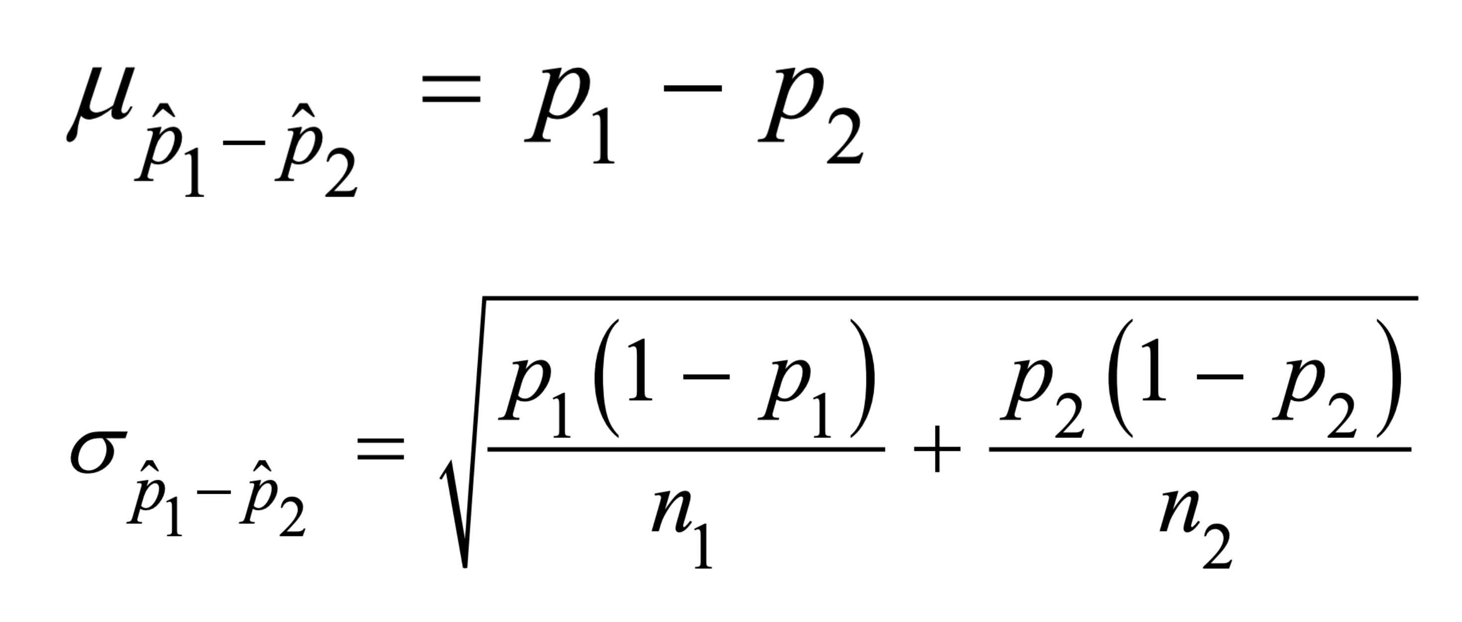
• The mean of the distribution of p̂₁ - p̂₂ is the difference in population proportions: μ(p̂₁-p̂₂) = p₁ - p₂.
• The standard deviation is σ(p̂₁-p̂₂) = √(p₁(1-p₁)/n₁ + p₂(1-p₂)/n₂). Variances add, then take the square root.
• The model is approximately normal only when all four counts are large: n₁p₁ ≥ 10, n₁(1-p₁) ≥ 10, n₂p₂ ≥ 10, n₂(1-p₂) ≥ 10.
• For proportions you check the large-counts (success-failure) condition, not the Central Limit Theorem. CLT applies to means.
• The two samples must come from two independent populations.
• When sampling without replacement, the true standard deviation is slightly smaller, but the difference is negligible if each sample is less than 10% of its population.

How the Distribution Works

The phrase "variances add" is the key to all difference distributions. Even though you subtract the two sample proportions, you add their variances before taking a square root for the standard deviation.

Center (mean):

μ(p̂₁-p̂₂) = p₁ - p₂

Spread (standard deviation):

σ(p̂₁-p̂₂) = √(p₁(1-p₁)/n₁ + p₂(1-p₂)/n₂)

Each piece p(1-p)/n is the variance of one group's sample proportion. You add those two variances, then square root the total. Some people call this the "Pythagorean Theorem of statistics" because you combine two squared pieces under a single square root.

Shape: The distribution of p̂₁ - p̂₂ is approximately normal when all four of these are met:

• n₁p₁ ≥ 10
• n₁(1 - p₁) ≥ 10
• n₂p₂ ≥ 10
• n₂(1 - p₂) ≥ 10

If any expected count falls below 10, the distribution can be skewed and the normal model may not be safe.

Source: AP Statistics Formula Sheet

This notation table is worth saving for quick reference.

How to Use This on the AP Statistics Exam

Problem Solving

1. Identify the two population proportions and sample sizes.

2. Find the center: p₁ - p₂.

3. Find the spread by adding the two variances p(1-p)/n, then square rooting.

4. Check all four large-counts conditions to confirm approximate normality.

5. If a probability is asked, standardize the observed difference with a z-score and use the normal model.

6. Interpret your answer in context, with units and a clear reference to both populations.

Common Trap

A frequent mistake is taking the square root of each group separately and then adding the standard deviations. That is wrong. You must add the variances first, then take one square root of the total.

Practice Problem

Suppose you are comparing the proportion of people in two cities who support a new public transportation system. You use simple random samples of 1000 people from each city. You find that 600 of the 1000 respondents from City A support the system, and 700 of the 1000 respondents from City B support the system.

a) Calculate the sample proportions of respondents who support the new system in each city.

b) Explain what the sampling distribution for the difference in sample proportions represents and why it is useful here.

c) Suppose the true population proportion in City A is 0.6 and in City B is 0.7. Describe the shape, center, and spread of the sampling distribution for the difference in sample proportions.

d) Explain why the difference in sample proportions can be modeled as approximately normal in this situation.

e) Discuss one potential source of bias that could affect the results, and explain how it could influence the estimate. (Hint: think about how this differs when working with two samples instead of one.)

Answer

a) City A: 600/1000 = 0.6. City B: 700/1000 = 0.7.

b) The sampling distribution for the difference in sample proportions represents the distribution of possible values of p̂₁ - p̂₂ if the study were repeated many times. It is useful because it lets you make inferences about the difference between the two population proportions based on the sample data.

c) If you define the difference as City A minus City B, the center is 0.6 - 0.7 = -0.1. If you define it as City B minus City A, the center is 0.7 - 0.6 = 0.1. The spread is the same either way: √(0.6(0.4)/1000 + 0.7(0.3)/1000) ≈ √(0.00024 + 0.00021) ≈ 0.0212. The shape is approximately normal because all four large-counts conditions are met.

d) All four expected counts are large: 1000(0.6) = 600, 1000(0.4) = 400, 1000(0.7) = 700, and 1000(0.3) = 300, all well above 10. With large counts satisfied for both groups, the distribution of p̂₁ - p̂₂ is approximately normal.

e) Nonresponse bias is one possibility. If supporters in City A are more likely to respond, that sample could overestimate support there. If people in City B who oppose the system are more likely to respond, that sample could underestimate support there. With two samples, bias in either group can distort the estimated difference, so you have to watch the response patterns in both cities, not just one.

Common Misconceptions

• Adding standard deviations instead of variances. Always add the two variances p(1-p)/n first, then square root once. Standard deviations do not add directly.
• Using the Central Limit Theorem for proportions. For proportions, you confirm normality with the large-counts (success-failure) checks. CLT is the justification you use for sample means.
• Checking only one group's counts. All four conditions must pass: both successes and failures, for both groups.
• Forgetting the independence requirement. The two samples must come from two independent populations for these formulas to apply.
• Ignoring the without-replacement adjustment. If a sample is 10% or more of its population, the true standard deviation is smaller than the formula gives. Below 10%, you can ignore the difference.
• Treating the sign of the difference as fixed. p̂₁ - p̂₂ and p̂₂ - p̂₁ have the same spread but opposite-signed centers. Be consistent about which group you label first.

Related AP Statistics Guides

• Unit 5 Overview: Sampling Distributions
• 5.1 Introducing Statistics: Why Is My Sample Not Like Yours?
• 5.5 Sampling Distributions for Sample Proportions
• 5.2 The Normal Distribution, Revisited
• 5.3 The Central Limit Theorem
• 5.4 Biased and Unbiased Point Estimates