A random variable is a variable that can take on different numerical values depending on the outcome of a random event. The probability distribution of a random variable specifies the probabilities of each possible value that the random variable can take on. It's common to use capital letters to represent random variables, such as X or Y.
Types of Random Variables
A discrete random variable can only take on a finite or countably infinite number of possible values of X. The probability of a discrete random variable is typically associated with individual values, rather than intervals, because the random variable can only take on specific, discrete values. Examples of discrete random variables include the number of heads that appear when flipping a coin three times, or the number of cars that pass through a particular intersection in a given hour.
A continuous random variable, on the other hand, can take on any value within a certain range. Generally, you use a density curve to find the probability of a continuous variable and the probability usually applies to an interval rather than individual values. Examples of continuous random variables include the height of a person, or the time it takes for a runner to complete a race.
To find the probability of a particular value or range of values for a continuous random variable, you can use a probability density function (PDF), which is beyond the scope of AP Stats (phew!). The probability of a continuous random variable is typically associated with an interval of values, rather than individual values, because it is possible for the random variable to take on any value within a certain range.
In both cases, the probabilities of all possible values of the random variable must sum to 1, as there is always a certain probability of some outcome occurring.

Probability Distributions = Best Friend!
When calculating probability for discrete random variables, it's helpful to know whether you should include the boundary value in your calculations. This is because the wording of the problem can sometimes be confusing and you may need to determine whether the boundary value is included or excluded.
For example, if you are asked to calculate the probability that a discrete random variable X takes on a value of "at least 3," you would need to include the value of 3 in your calculations. Similarly, if you are asked to calculate the probability that X takes on a value of "no more than 3," you would need to include the value of 3 in your calculations.
One way to help clarify these types of problems is to draw a mini probability distribution chart that shows all of the possible values of the random variable X and their probabilities. This can help you visualize the problem and make it easier to determine which values to include or exclude in your calculations on top of phrases like at least, no more than, greater than, etc.
To calculate the probability of a discrete random variable X taking on a particular value n, you can use the formula P(X = n) or P(Xn). This formula gives you the probability of the random variable X taking on the value n. You can then use this probability to answer the question or solve the problem you are working on.
A sample probability distribution chart is shown below:
| Value | x1 | x2 | x3 | x4 |
|---|---|---|---|---|
| Probability | p1 | p2 | p3 | p4 |
You need to know how to represent a discrete random variable as a histogram or in a table. For the histogram, use the discrete random variable as the x-axis values and the probabilities for the y-axis values.
Interpretation & Context
When describing the shape of a discrete random variable, it can be helpful to talk about whether the graph is roughly symmetric, double-peaked, or single-peaked, as well as whether it is right-skewed or left-skewed. These characteristics can give you insights into the underlying probability distribution of the random variable.
Here are examples of conclusions drawn from the shape of a graph of a discrete random variable:
- If the graph of a discrete random variable is roughly symmetric, it means that the values of the random variable are evenly distributed around the center of the distribution. This often indicates that the distribution is normal, or bell-shaped.
- If the graph of a discrete random variable is double-peaked, it means that there are two distinct peaks in the distribution. This often indicates that there are two distinct groups of values that the random variable can take on.
- If the graph of a discrete random variable is single-peaked, it means that there is only one peak in the distribution. This can indicate that there is a dominant group of values that the random variable is more likely to take on.
- If the graph of a discrete random variable is right-skewed, it means that the values are concentrated on the left side of the distribution, with a long tail extending to the right. This often indicates that the distribution is skewed towards lower values.
- If the graph of a discrete random variable is left-skewed, it means that the values are concentrated on the right side of the distribution, with a long tail extending to the left. This often indicates that the distribution is skewed towards higher values.
In addition to describing the shape of the distribution, it's also important to mention the center (mean) and measure of variability (standard deviation) of the distribution. These values can help you make conclusions about the distribution and how the values of the random variable are likely to behave. For example, the mean of the distribution can give you an idea of the most likely value that the random variable will take on, while the standard deviation can give you an idea of how spread out the values of the random variable are.
🎥 Watch: AP Stats - Probability: Random Variables, Binomial/Geometric Distributions
Example
A recent study found that the probability that a person will develop a certain type of cancer is 0.01. This probability is independent of all other persons. The table below shows the number of people in a group of 10 people and the probability that exactly that number of people in the group will develop this type of cancer:

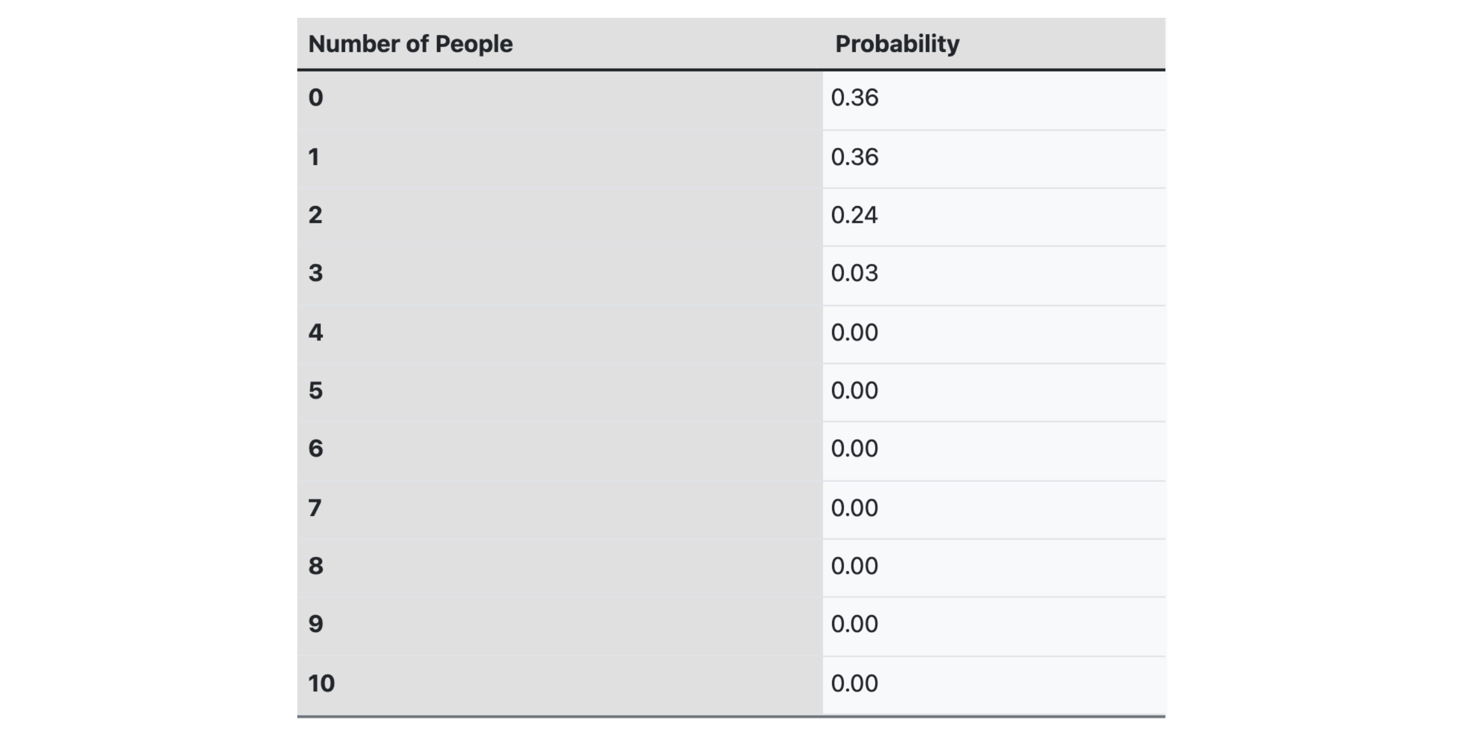
(a) What is the probability that at least 5 of a group of 10 people will develop this type of cancer?
(b) What is the probability that no more than 3 of a group of 10 people will develop this type of cancer?
(c) What is the probability that at most 2 of a group of 10 people will develop this type of cancer?
Answer
(a) To find the probability that at least 5 of a group of 10 people will develop this type of cancer, you will need to find the probability that exactly 5 people in the group will develop the cancer, plus the probability that exactly 6 people in the group will develop the cancer, plus the probability that exactly 7 people in the group will develop the cancer, and so on. You can do this by looking up the probabilities in the table and adding them all together.
P(X > 5) = 0.00 + 0.00 + 0.00 + 0.00 + 0.00 = 0.00
The probability that at least 5 of a group of 10 people will develop this type of cancer is 0.00.
(b) The probability that no more than 3 of a group of 10 people will develop this type of cancer is 0.99. This is calculated by adding the probabilities of exactly 0 people in the group developing cancer (0.36), exactly 1 person in the group developing cancer (0.36), exactly 2 people in the group developing cancer (0.24), and exactly 3 people in the group developing cancer (0.03).
P(X ≤ 3) = P(X = 0) + P(X = 1) + P(X = 2) + P(X=3) = 0.36 + 0.36 + 0.24 + 0.03= 0.99
The probability that no more than 3 of a group of 10 people will develop this type of cancer is 0.99.
(c) The probability that at most 2 of a group of 10 people will develop this type of cancer is 0.96. This is calculated by adding the probabilities of exactly 0 people in the group developing cancer (0.36), exactly 1 person in the group developing cancer (0.36), and exactly 2 people in the group developing cancer (0.24).
P(X ≤ 2) = P(X = 0) + P(X = 1) + P(X = 2) = 0.36 + 0.36 + 0.24 = 0.96
The probability that at most 2 of a group of 10 people will develop this type of cancer is 0.96.
Vocabulary
The following words are mentioned explicitly in the College Board Course and Exam Description for this topic.
| Term | Definition |
|---|---|
| center | A measure indicating the middle or typical value of a distribution. |
| cumulative probability distribution | A representation (as a table or function) showing the probability that a random variable is less than or equal to each of its possible values. |
| discrete random variable | A random variable that takes on a countable number of distinct values, often representing counts or categorical outcomes. |
| population | The entire group of individuals or items from which a sample is drawn and about which conclusions are to be made. |
| probability distribution | A function that describes the likelihood of all possible values of a random variable. |
| random process | A process that generates results determined by chance, where the outcome cannot be predicted with certainty in advance. |
| random variable | A variable whose value is determined by the outcome of a random phenomenon and can take on different numerical values with associated probabilities. |
| shape | The overall form or pattern of a distribution, including characteristics like skewness and modality. |
| spread | A measure of how dispersed or variable the outcomes of a probability distribution are, such as range, variance, or standard deviation. |
Frequently Asked Questions
What's the difference between a random variable and a regular variable in math?
A regular variable in algebra is just a symbol that can stand for any number you choose or solve for—it's deterministic: x = 5 or x could be any real number in an equation. A random variable, however, represents the numerical outcome of a random process: its value is not fixed until you observe it. For AP Stats (Topic 4.7) focus on discrete random variables: they have a list (support) of possible values and a probability mass function (pmf) giving P(X = x) for each value; those probabilities must sum to 1 (VAR-5.A). You use the distribution (table, graph, or function) to find probabilities, cumulative probabilities (cdf), the expected value E(X)=Σ x·P(x), and variance. Random variables link probability theory to data—they appear on the exam in distribution/expected-value questions. For a quick review, see the Topic 4.7 study guide (https://library.fiveable.me/ap-statistics/unit-4/intro-random-variables-probability-distributions/study-guide/B5MJ1YqQJ4D455wegCvz) and try practice problems (https://library.fiveable.me/practice/ap-statistics).
How do I know if a random variable is discrete or continuous?
Look for whether the possible outcomes are countable or form an interval. - Discrete: takes a countable set of values (often counts). Each value has a probability and the probabilities sum to 1. Examples: number of puppies in a litter, sum when rolling two dice, count of successes (binomial). You’d represent it with a probability mass function (pmf), table, or histogram (CED VAR-5.A). - Continuous: can take any value in an interval (measurements). Probabilities for exact single values are 0; you find probabilities for ranges (areas under a density curve). Examples: a penguin’s weight or time until relief from a headache. Quick test: if you can list or enumerate all possible outcomes (0,1,2,…) it’s discrete; if outcomes fill an interval (any real number in a range), it’s continuous. For AP practice and examples, see the Topic 4.7 study guide (https://library.fiveable.me/ap-statistics/unit-4/intro-random-variables-probability-distributions/study-guide/B5MJ1YqQJ4D455wegCvz), unit overview (https://library.fiveable.me/ap-statistics/unit-4), and practice problems (https://library.fiveable.me/practice/ap-statistics).
What does it mean when they say the sum of all probabilities must equal 1?
It means the probability distribution lists every possible value a discrete random variable can take and assigns each a probability so that the total chance of all possible outcomes equals 1 (the “normalization” condition in the CED, VAR-5.A.2). Why? Because when you run the random process once, something in the support has to happen—the probabilities represent the long-run relative frequencies of those outcomes, and their sum is the certainty (100% → 1). Example: rolling one fair die has outcomes 1–6, each with probability 1/6; 6 × (1/6) = 1. For a binomial X ~ Bin(n,p), summing P(X = x) over x = 0…n gives 1. On the AP exam you may be asked to check that a PMF is valid by showing all probabilities are nonnegative and sum to 1 (Topic 4.7, VAR-5.A). For a quick refresher, see the Topic 4.7 study guide (https://library.fiveable.me/ap-statistics/unit-4/intro-random-variables-probability-distributions/study-guide/B5MJ1YqQJ4D455wegCvz) and try practice problems (https://library.fiveable.me/practice/ap-statistics).
How do I make a probability distribution table from scratch?
Start by listing the possible values (the support) of your discrete random variable—e.g., 0,1,2,3. For each value, find P(X = x) using logic, counting, or a formula (binomial: P(X=x)=C(n,x)p^x(1−p)^(n−x)). Put those in a two-row table: x across the top and P(x) below (this is the pmf). Check the normalization condition: all probabilities must be ≥0 and sum to 1. If asked, add a cumulative column P(X ≤ x) to make a cdf table. Finally compute mean and variance if needed: E(X)=Σ x·P(x) and Var(X)=Σ (x−E(X))^2·P(x). On the AP exam you can present distributions as a table, graph, or function—make sure you label units and context (CED VAR-5.A). Want practice? See the Topic 4.7 study guide (https://library.fiveable.me/ap-statistics/unit-4/intro-random-variables-probability-distributions/study-guide/B5MJ1YqQJ4D455wegCvz) and more practice problems (https://library.fiveable.me/practice/ap-statistics).
I don't understand what a cumulative probability distribution is - can someone explain?
A cumulative probability distribution (or cumulative distribution function, CDF) for a discrete random variable X gives, for each value x, the probability that X is less than or equal to x: P(X ≤ x). It’s different from the probability mass function (pmf), which lists P(X = x) for each x. The CDF is built by adding up the pmf values up to each x, so the final value (largest x) equals 1 (normalization). Why it’s useful: you can read off medians and percentiles directly (median is the smallest x with CDF ≥ 0.5), compute probabilities like P(a < X ≤ b) by subtracting CDFs, and compare distributions’ centers/spread—skills tied to VAR-5.A in Topic 4.7. Example: if X = sum of two dice, the CDF at 7 is P(X ≤ 7) = sum of pmf for 2–7. For more practice and AP-aligned explanation, check the Topic 4.7 study guide (https://library.fiveable.me/ap-statistics/unit-4/intro-random-variables-probability-distributions/study-guide/B5MJ1YqQJ4D455wegCvz) and Unit 4 overview (https://library.fiveable.me/ap-statistics/unit-4). For lots of practice problems, see (https://library.fiveable.me/practice/ap-statistics).
When do I use a graph vs a table vs a function to show probability distributions?
Use a table when you want exact probabilities listed for each possible value—that’s the most straightforward representation of a discrete random variable’s pmf (good for n small, shows P(X = x) explicitly and makes it easy to check the normalization condition ΣP(x)=1). Use a probability histogram (graph) when you want to show shape, center, and spread visually—it’s great for comparing distributions (AP calls this a probability histogram). Use a function (pmf or formula) when probabilities follow a rule (e.g., binomial P(X=x)=C(n,x)p^x(1−p)^{n−x}); a function is compact and necessary on the exam when you’re asked to derive probabilities or expectations. For cumulative info use a cdf/table of P(X≤x) (CED VAR-5.A.4). Remember: tables/functions give exact values; graphs reveal shape and help interpret center/spread (VAR-5.B). For a quick refresher see the Topic 4.7 study guide (https://library.fiveable.me/ap-statistics/unit-4/intro-random-variables-probability-distributions/study-guide/B5MJ1YqQJ4D455wegCvz) and Unit 4 overview (https://library.fiveable.me/ap-statistics/unit-4). For extra practice, try problems at (https://library.fiveable.me/practice/ap-statistics).
What's the formula for finding the probability of a discrete random variable?
For a discrete random variable X the probability is given by its probability mass function (pmf): p(x) = P(X = x). Two requirements: 0 ≤ p(x) ≤ 1 for every possible x, and Σ p(x) over all x in the support = 1 (VAR-5.A.2–3). Common useful formulas you should memorize from the CED/formula sheet: - General pmf: p(x) = P(X = x). - Mean (expected value): μX = E(X) = Σ x·p(x). - If X ~ Binomial(n, p): P(X = k) = C(n, k) p^k (1 − p)^(n−k), k = 0,1,...,n (used often on the AP exam; see Topic 4.7 and Unit 4 weighting). Want quick practice and cheat-sheet review? Check the Topic 4.7 study guide (https://library.fiveable.me/ap-statistics/unit-4/intro-random-variables-probability-distributions/study-guide/B5MJ1YqQJ4D455wegCvz) and try problems at https://library.fiveable.me/practice/ap-statistics.
How do I solve problems about rolling dice and finding probability distributions?
Think of a die roll as a discrete random variable (VAR-5.A): list the numeric outcomes, give each outcome’s probability (pmf), and check they sum to 1. Quick steps for dice problems: 1. Define the random variable X (e.g., sum of two fair dice). 2. List the sample space and count equally likely outcomes (two dice → 36 total). 3. Find P(X = x) for each x (make a table or histogram per VAR-5.A.3). 4. Check normalization: ΣP = 1. 5. Compute E(X)=Σ x·P(x) and Var(X)=Σ (x−E(X))^2·P(x) if asked. Example: two fair dice sums: P(2)=1/36, P(3)=2/36, P(4)=3/36, …, P(7)=6/36, …, P(12)=1/36. Expected sum E(X)=7. On the AP exam you may be asked to represent the pmf as a table/graph, interpret shape/center/spread (VAR-5.B), or compute expected value/variance. For more practice and guided examples, see the Topic 4.7 study guide (https://library.fiveable.me/ap-statistics/unit-4/intro-random-variables-probability-distributions/study-guide/B5MJ1YqQJ4D455wegCvz) and Unit 4 resources (https://library.fiveable.me/ap-statistics/unit-4).
What's the difference between P(X = k) and P(X ≤ k) in probability?
P(X = k) is the probability the discrete random variable X takes the single value k—that’s the probability mass function (pmf). P(X ≤ k) is the cumulative probability (cdf): the probability X is k or any value less than k, i.e. the sum of the pmf for all values ≤ k. Quick example from Topic 4.7: for S ~ Binomial(n=3, p=0.8) we have P(S=2) = C(3,2)(0.8)^2(0.2) = 0.384. Then P(S ≤ 2) = P(0)+P(1)+P(2) = 0.008 + 0.096 + 0.384 = 0.488. So P(S=2) tells you the chance of exactly two successes; P(S≤2) tells you the chance of at most two successes. On the AP exam you should be able to represent both pmf and cdf (VAR-5.A.3 and VAR-5.A.4) and use whichever one fits the question. For more practice and explanations see the Topic 4.7 study guide (https://library.fiveable.me/ap-statistics/unit-4/intro-random-variables-probability-distributions/study-guide/B5MJ1YqQJ4D455wegCvz) and Unit 4 resources (https://library.fiveable.me/ap-statistics/unit-4).
I'm confused about how to interpret the shape, center, and spread of a probability distribution - what do these mean?
Shape, center, and spread describe different parts of a probability distribution so you can interpret it quickly. - Shape: how probabilities are arranged (symmetric, skewed right/left, unimodal, uniform). Shape tells you where most outcomes fall and whether tails are long (e.g., right skew means occasional large values). (CED: VAR-5.B.1; distributions can be shown as a pmf, histogram, or table—VAR-5.A.3.) - Center: a typical/average outcome. For a discrete random variable that’s the expected value E(X) = Σ x·P(x) (CED: expected value in keywords). The center helps you predict the long-run average outcome. - Spread: how much outcomes vary (variance or standard deviation for a distribution, or range/IQR graphically). Bigger spread means more variability around the center; smaller spread means outcomes cluster tightly. On the AP exam you’ll be asked to describe these in context (mention units, compare distributions, and use terms like expected value or variance). For a focused review see the Topic 4.7 study guide (https://library.fiveable.me/ap-statistics/unit-4/intro-random-variables-probability-distributions/study-guide/B5MJ1YqQJ4D455wegCvz) and more practice at (https://library.fiveable.me/practice/ap-statistics).
How do I calculate cumulative probabilities step by step?
Step-by-step for cumulative probabilities (CDF) with a discrete random variable: 1. Identify the random variable X and its possible values (support) and write the probability mass function (pmf) as a table or list. 2. Order the values of X from smallest to largest. 3. For each value x, compute the cumulative probability P(X ≤ x) by summing the pmf for all values ≤ x: P(X ≤ x) = Σ P(X = k) for k ≤ x. Do this sequentially so each cumulative entry adds the next pmf. 4. Put these P(X ≤ x) values in a cumulative table or plot the CDF (step function). 5. Check that the final cumulative probability = 1 and every pmf entry is between 0 and 1. 6. If the distribution is a known model (e.g., binomial), use formulas or a calculator command (binomcdf) to get cumulative probabilities quickly—useful on the AP when n is large. This matches VAR-5.A and VAR-5.A.4 in the CED. For examples and practice, see the Topic 4.7 study guide (https://library.fiveable.me/ap-statistics/unit-4/intro-random-variables-probability-distributions/study-guide/B5MJ1YqQJ4D455wegCvz) and more problems (https://library.fiveable.me/practice/ap-statistics).
Can someone walk me through creating a probability distribution for the number of puppies in a litter?
Think of X = number of puppies in a randomly selected litter. X is a discrete random variable (VAR-5.A). To create its probability distribution you need the possible values and probabilities that sum to 1. Steps: 1. Choose the support (realistic values): e.g., X = 0,1,2,3,4,5. 2. Get probabilities from data (best) or a model. If you have breeder records, compute P(X = k) = (count of litters with k pups)/(total litters). If you don’t have data, say a plausible model but note it must be justified—litter size usually isn’t binomial, so don’t assume binomial without checking. 3. Make a table or pmf: k: 0 1 2 3 4 5 P(k): 0.01 0.05 0.20 0.40 0.25 0.09 (example; must sum to 1) 4. Check normalization: sum P(k)=1. 5. (Optional) Compute E(X)=Σ k·P(k) and Var(X)=Σ (k−E)^2·P(k). Interpret E(X) as the long-run average litter size (VAR-5.C). On the AP exam you may be asked to represent the pmf as a table/graph and interpret center/spread (VAR-5.A, VAR-5.B). For a concise walk-through and examples, see the Topic 4.7 study guide (https://library.fiveable.me/ap-statistics/unit-4/intro-random-variables-probability-distributions/study-guide/B5MJ1YqQJ4D455wegCvz) and unit overview (https://library.fiveable.me/ap-statistics/unit-4). For extra practice problems, try (https://library.fiveable.me/practice/ap-statistics).
What does it mean for a random variable to have "countable" values?
“Countable” means you can list the possible values of the random variable one-by-one (even if the list is very long). In AP terms a discrete random variable takes a countable set of values and each value has a probability (VAR-5.A.2). That includes finite sets (0,1,2,3 puppies) and countably infinite sets (1,2,3,… like the number of tosses until first heads). It excludes uncountable ranges (like every real number between 0 and 1)—those are continuous. For discrete variables you give a probability mass function (pmf), a table, or a histogram showing probabilities over the variable’s support; the probabilities must sum to 1 (VAR-5.A.3, VAR-5.A.2). For more AP-aligned examples and practice, see the Topic 4.7 study guide (https://library.fiveable.me/ap-statistics/unit-4/intro-random-variables-probability-distributions/study-guide/B5MJ1YqQJ4D455wegCvz) and the Unit 4 overview (https://library.fiveable.me/ap-statistics/unit-4). For extra practice problems, try (https://library.fiveable.me/practice/ap-statistics).
How do I check if my probability distribution is valid or correct?
To check a discrete probability distribution is valid, do these quick checks: 1. List the support (all possible values of the random variable). A discrete RV must have a countable set of values (e.g., 0,1,2,...). 2. Check each probability: 0 ≤ P(x) ≤ 1 for every value x. 3. Normalization: add all P(x) for every value in the support—the sum must equal 1 (this is the CED VAR-5.A.2 requirement). 4. If you have a cumulative distribution (CDF), ensure it’s nondecreasing and approaches 1 as x goes to the max. 5. If you claim a named model (e.g., binomial), verify its parameter conditions (n integer ≥0, 0≤p≤1) and that P(x) matches the pmf formula. If something fails (sum ≠ 1 or a negative/>1 probability), the distribution is invalid. For more examples and practice problems on Topic 4.7, see the Fiveable study guide (https://library.fiveable.me/ap-statistics/unit-4/intro-random-variables-probability-distributions/study-guide/B5MJ1YqQJ4D455wegCvz) and try problems at (https://library.fiveable.me/practice/ap-statistics).
Why do all the probabilities in a discrete distribution have to add up to exactly 1?
Think of a probability distribution as a complete description of every possible outcome for a random process. If X is a discrete random variable, VAR-5.A.2 in the CED says each possible value x has a probability P(X = x), and those probabilities must sum to 1—that’s the normalization condition. Why exactly? Because “1” means certainty: across all possible outcomes one of them has to happen. Adding the probabilities over the whole sample space gives the probability that some outcome occurs, so that total must be 1 (100% chance something in the sample space happens). On the AP exam you’ll need to show you can list the support and check the probabilities sum to 1 (VAR-5.A, skill 2.B). For extra practice and examples on discrete pmfs and binomial/cumulative tables, see the Topic 4.7 study guide (https://library.fiveable.me/ap-statistics/unit-4/intro-random-variables-probability-distributions/study-guide/B5MJ1YqQJ4D455wegCvz) and try problems at (https://library.fiveable.me/practice/ap-statistics).