When given a statistical claim from an article or previous study, the first necessary thing to do is to identify the test needed. Some key phrases you will see that tells us that a statistical significance test is called for is "do the data give convincing evidence..." or "is there convincing evidence of..." 🤔
When one of these key phrases appear in the prompt, we then need to determine if our data is categorical data or quantitative data. If we have quantitative data, we will set up a test for a population mean. As with confidence intervals, a test for population mean will make use of t-scores. If we only have one sample, we will perform a one sample t-test.
A one-sample t-test is used to compare the mean of a sample to a known population mean. It is often used when the standard deviation (σ) of the population is not known. To conduct a one-sample t-test, you first need to determine the null and alternative hypotheses. The null hypothesis is a statement of no difference or no effect, and it is the hypothesis that is being tested, while the alternative hypothesis is the opposite of the null hypothesis, and it is what you hope to show is true. 1️⃣
Significance Level
One major aspect of our significance test is the significance level. The significance level (alpha, 𝞪) is the probability of rejecting the null hypothesis when it is actually true. It is the threshold that you set for determining whether the sample mean is significantly different from the claimed population mean. If the p-value is less than the significance level, then you can reject the null hypothesis and conclude that the sample mean is significantly different from the claimed population mean. 🔝
It's important to choose an appropriate significance level because setting it too low can lead to a high rate of false positives (also known as Type I errors), where you reject the null hypothesis when it is actually true. On the other hand, setting it too high can lead to a high rate of false negatives (also known as Type II errors), where you fail to reject the null hypothesis when it is actually false.
The most common significance level used in research is 0.05, which means that there is a 5% chance of rejecting the null hypothesis when it is actually true. This is often considered a good balance between minimizing the risk of Type I and Type II errors. However, the appropriate significance level will depend on the specific research question and the context in which the research is being conducted.

Connection to Confidence Interval
A significance level is directly connected to a one sample t-interval. If we have a significance level of 0.05, we would be looking at a sample statistic that would not occur in our 95% confidence interval. If we select a significance level of 0.02, it matches with a 98% confidence interval. In summation, the complement of our significance level will match with the confidence level of the matching confidence interval. 🌉
Example
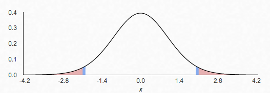
In the image below, we see a 95% confidence interval in the non-shaded region for a mean of 0 and 29 df. The shaded region is known as the rejection region. This is the region in which a statistic is significant enough (in accordance with its 𝞪 level) to reject the claimed population mean. In this example, any sample statistic greater than 2.04 or less than -2.04 would lead us to doubt that the true population mean is 0. 🙅
image created with: https://homepage.divms.uiowa.edu/~mbognar/Writing Hypotheses
Once we have identified our test and significance level, we need to identify and write our hypothesized values. We have two hypotheses: null and alternate.
Null Hypothesis (Ho)
In a one-sample t-test, the null hypothesis is a statement about the population mean, and it is based on the claim made by the previous study or article. The null hypothesis is typically stated as 𝞵 = μ0, where 𝞵 is the sample mean and μ0 is the hypothesized population mean. 🥚
For example, if the previous study claimed that the mean number of chicken nuggets per bag is 20, the null hypothesis for a one-sample t-test would be 𝞵 = 20. This means that the null hypothesis is that the true mean number of chicken nuggets per bag is equal to 20.
Our null hypothesis is always going to be 𝞵 = hypothesized population mean (in number format).
Down the road, the purpose of the one-sample t-test is to determine whether the sample mean is significantly different from the hypothesized population mean. If the p-value is less than the predetermined significance level (usually 0.05), then you can reject the null hypothesis and conclude that the sample mean is significantly different from the hypothesized population mean. If the p-value is greater than the significance level, then you cannot reject the null hypothesis, and you must accept the claim as being true.
Alternate Hypothesis (Ha)
The alternative hypothesis is the opposite of the null hypothesis, and it is what you hope to show is true. In a one-sample t-test, the alternative hypothesis can take one of three forms: 𝞵 ≠ μ0, 𝞵 < μ0, or 𝞵 > μ0, where 𝞵 is the sample mean and μ0 is the hypothesized population mean from the null hypothesis. 🐤
For example, if the null hypothesis is 𝞵 = 20 (the hypothesized population mean is 20), the alternative hypothesis could be 𝞵 ≠ 20 (the sample mean is not equal to 20), 𝞵 < 20 (the sample mean is less than 20), or 𝞵 > 20 (the sample mean is greater than 20).
The alternative hypothesis that you choose will depend on the specific research question and the context in which the research is being conducted. For example, if you are testing the claim that the mean number of chicken nuggets per bag is 20, and you expect the actual mean to be higher, you would choose the alternative hypothesis 𝞵 > 20. On the other hand, if you expect the actual mean to be lower, you would choose the alternative hypothesis 𝞵 < 20.
Example
A recent study has found that the average number of school days missed by a high school senior is 5.2 days. After taking a random sample of 150 high school seniors, our sample has an average of 4.1 days missed with a standard deviation of 0.4. Do the data give convincing evidence that the average number of days missed by a high school senior is less than the claim from the study?
- Ho: 𝞵 = 5.2
- Ha: 𝞵 < 5.2
For this example, our null hypothesis comes directly from the study. The alternative hypothesis comes from the fact that the question implies that we are checking to see if the actual value is less than the hypothesized value.
Checking Conditions
Once we have our test confirmed and our hypothesis developed, we need to check our conditions for inference to be sure that our test can accurately be carried out. Just as with confidence intervals, we have 3 conditions: 🧪
- Random
- Independent
- Normal
Random
If we are planning on using our sample statistics to develop a statistical test, it is imperative that our sample was chosen randomly. This is important because we are planning on using our sample mean to draw inference or conclusions about our population mean. 🍀
If our sample is not chosen randomly to mirror our population, we cannot make statistical claims about the given population.
Independence
Since we are more than likely sampling without replacement, our sample is not truly independent. However, if our sample is not super close to the population, the effect of sampling without replacement is said to be negligible enough that our sample is essentially independent. 🏁
To check that this condition is met, we must verify that it is reasonable to believe that our population is at least 10x that of our sample.
You should state, "It is reasonable to believe that there are ____ (10n) _________ (in context of our population)"
Normal
Since we will be using the normal curve in our next unit to actually calculate the values necessary to perform our test, we need to assure that our sampling distribution is approximately normal. 🔔
There are three options to check this:
- Central Limit Theorem (sample size is at least 30)
- Population is given to be approximately normal.
- Distribution of sample data looks approximately symmetric with no apparent outliers or gaps. This can be shown with a quick, modified box-plot sketch of our sample data. Checking these conditions in this order will be the least cumbersome attempt in verifying the normal condition. Only one is necessary to verify normality.
🎥 Watch: AP Stats - Inference: Hypothesis Tests for Means
Vocabulary
The following words are mentioned explicitly in the College Board Course and Exam Description for this topic.
| Term | Definition |
|---|---|
| 10% condition | The requirement that sample size n is at most 10% of the population size N to ensure independence when sampling without replacement. |
| alternative hypothesis | The claim that contradicts the null hypothesis, representing what the researcher is trying to find evidence for. |
| approximately normal | A distribution that closely follows the shape of a normal distribution, allowing for the use of normal probability methods. |
| conditions for the test | The requirements that must be satisfied before conducting a hypothesis test for a population mean, including independence and normality of the sampling distribution. |
| independence | The condition that observations in a sample are not influenced by each other, typically ensured through random sampling or randomized experiments. |
| matched pairs | Paired observations where two measurements are taken on the same subject or on subjects that are matched according to specific criteria, used to analyze the mean difference between the paired values. |
| mean difference | The average of the differences between paired observations, denoted by μd, where the order of subtraction must be clearly defined. |
| null hypothesis | The initial claim or assumption being tested in a hypothesis test, typically stating that there is no effect or no difference. |
| one-sample t-test | A hypothesis test used to determine whether a population mean differs from a hypothesized value when the population standard deviation is unknown. |
| outlier | Data points that are unusually small or large relative to the rest of the data. |
| population mean | The average of all values in an entire population, denoted as μ. |
| population means | The average values of two distinct populations being compared, denoted as μ₁ and μ₂. |
| random sample | A sample selected from a population in such a way that every member has an equal chance of being chosen, reducing bias and allowing for valid statistical inference. |
| randomized experiment | A study design where subjects are randomly assigned to treatment groups to establish cause-and-effect relationships. |
| sample size | The number of observations or data points collected in a sample, denoted as n. |
| sampling distribution | The probability distribution of a sample statistic (such as a sample proportion) obtained from repeated sampling of a population. |
| sampling without replacement | A sampling method in which an item selected from a population cannot be selected again in subsequent draws. |
| significance test | A statistical procedure used to determine whether there is sufficient evidence to reject the null hypothesis based on sample data. |
| skewness | A measure of the asymmetry of a distribution, indicating whether data is concentrated more on one side of the center. |
Frequently Asked Questions
How do I know when to use a one-sample t-test instead of a z-test for population means?
Use a one-sample t-test when you’re testing a population mean and the population standard deviation σ is unknown (CED VAR-7.B.1). Replace σ with the sample s and use the t-distribution with df = n − 1 to compute the t-statistic and p-value. Use a z-test only when σ is known (rare on the AP exam). Before you proceed, check the t-test conditions (CED VAR-7.D): data from a random sample or randomized experiment, n ≤ 10% of the population if sampling without replacement, and the sampling distribution of x̄ approx. normal—if n < 30 make sure the sample data show no strong skewness or outliers; if n ≥ 30 the CLT helps. For matched pairs, compute differences and do a one-sample t on the mean difference μd (CED VAR-7.B.2 and VAR-7.C.2). For the AP exam, you’ll use the t table/formulas provided; review Topic 7.4 on Fiveable (study guide: https://library.fiveable.me/ap-statistics/unit-7/setting-up-test-for-population-mean/study-guide/1gAGgo2P3abc5G0sLvMr) and practice problems (https://library.fiveable.me/practice/ap-statistics).
What's the difference between a t-test and a z-test when testing population means?
Short answer: use a z-test when the population standard deviation σ is known; use a t-test when σ is unknown and you estimate it with the sample standard deviation s. Why it matters (AP CED facts): VAR-7.B.1 says a one-sample t-test is the appropriate test for a population mean when σ is unknown. The t-statistic is t = (x̄ − μ0) / (s/√n) with degrees of freedom df = n − 1. The t-distribution is like the normal (z) but has thicker tails—that means larger critical values (especially for small n), so your test is more conservative when n is small. As n grows (≈30+), the t-distribution approaches the normal, so z and t give similar results. Also: matched pairs are handled by a paired t-test on the differences (define order of subtraction). Always check independence (random sample, 10% condition) and approximate normality (no strong skew/outliers for n<30) per VAR-7.D.1–D.2. AP exam supplies t and z tables and lets you use a graphing calculator (see Unit 7 study guide (https://library.fiveable.me/ap-statistics/unit-7/setting-up-test-for-population-mean/study-guide/1gAGgo2P3abc5G0sLvMr) and unit overview (https://library.fiveable.me/ap-statistics/unit-7)). For extra practice, try the 1000+ problems at (https://library.fiveable.me/practice/ap-statistics).
I'm confused about matched pairs - how do I set up the hypotheses for the mean difference?
Think of matched pairs as one sample of differences: for each pair calculate d = (first − second) where you define the order and stick with it. Then do a one-sample t test on the differences. Hypotheses (using μd for the population mean difference): - H0: μd = 0 (or μd = μ0 if a nonzero value is hypothesized) - Ha (two-sided): μd ≠ 0 - Ha (one-sided): μd > 0 or μd < 0 The sign in Ha depends on your order of subtraction. Example: if d = after − before and you expect an increase, Ha: μd > 0. Remember conditions from the CED: data random/independent, n ≤ 10% of population if no replacement, and the distribution of the differences should be approximately normal (if n < 30) or not strongly skewed/no outliers. The test statistic is t = (d̄ − μd0)/(sd/√n) with df = n−1. For a quick review, see the Topic 7.4 study guide (https://library.fiveable.me/ap-statistics/unit-7/setting-up-test-for-population-mean/study-guide/1gAGgo2P3abc5G0sLvMr). For extra practice, try problems at (https://library.fiveable.me/practice/ap-statistics).
When do I use the 10% rule and what happens if my sample is bigger than 10% of the population?
Use the 10% rule whenever you sample without replacement from a finite population—it’s part of the independence check for a t-test (CED VAR-7.D.1). The rule says n ≤ 0.10·N. If your sample is ≤10% of the population, observations can be treated as (approximately) independent and the usual t procedures and SE = s/√n are OK. If your sample is >10% of the population, independence is violated: the usual standard error is too big a wiggle (you’re overcounting variability) and the t-test assumptions aren’t strictly met. Two practical fixes: - If N is known, apply the finite population correction (FPC) to the SE: SE_corrected = (s/√n)·√((N−n)/(N−1)). - If you can’t use FPC or the dependence is serious, you should avoid the standard t-test and either sample with replacement, use a different design (e.g., census), or explicitly account for the sampling design. For AP exam questions, always state you checked independence with the 10% condition; if it fails, say the t-procedure isn’t valid unless FPC is used (see the Topic 7.4 study guide on Fiveable) (https://library.fiveable.me/ap-statistics/unit-7/setting-up-test-for-population-mean/study-guide/1gAGgo2P3abc5G0sLvMr). For extra practice, try problems at (https://library.fiveable.me/practice/ap-statistics).
How do I check if my data is normal enough to use a t-test when n is less than 30?
When n < 30 you must check two things before using a one-sample (or paired) t-test: independence and approximate normality of the sampling distribution. - Independence: data from a random sample or randomized experiment; if sampling without replacement make sure n ≤ 10% of the population (10% condition). - Normality (shape): because CLT may not save you for small n, look at the raw data with a histogram, boxplot and a normal probability (QQ) plot. Check for strong skewness or outliers. If the distribution is roughly symmetric and free of strong outliers, the t-test is appropriate. If it’s strongly skewed or has outliers, don’t use the t; consider a larger sample, transform the data, or use a nonparametric method. AP note: the CED says for n < 30 the sample data should be free from strong skewness and outliers to verify the normality condition (VAR-7.D.1). For more guidance and examples see the Topic 7.4 study guide (https://library.fiveable.me/ap-statistics/unit-7/setting-up-test-for-population-mean/study-guide/1gAGgo2P3abc5G0sLvMr) and practice problems (https://library.fiveable.me/practice/ap-statistics).
What's the formula for setting up null and alternative hypotheses for a one-sample t-test?
For a one-sample t-test (σ unknown) you set the hypotheses about the population mean μ using the hypothesized value μ0: - Null: H0: μ = μ0 - Alternative (choose one based on the claim): Ha: μ < μ0 (left-tailed), Ha: μ > μ0 (right-tailed), or Ha: μ ≠ μ0 (two-tailed) If you’re doing matched pairs, form differences d = (first − second) and test about μd the same way (be explicit about the subtraction order). The test uses t = (x̄ − μ0) / (s/√n) with df = n − 1, and you must check independence and approximate normality (10% condition, and n>30 or no strong skew/outliers for small n) per the CED. For a quick refresher, see the Topic 7.4 study guide (https://library.fiveable.me/ap-statistics/unit-7/setting-up-test-for-population-mean/study-guide/1gAGgo2P3abc5G0sLvMr) and try practice problems (https://library.fiveable.me/practice/ap-statistics).
Can someone explain step by step how to do a matched pairs t-test?
Quick step-by-step for a matched-pairs (paired) t-test: 1. Define differences and order: for each pair compute d = (before − after) or whichever order makes sense; be consistent. Your parameter is μd (mean difference). 2. State hypotheses: H0: μd = 0 (or another value) and Ha: μd ≠ 0, < 0, or > 0 depending on the claim. 3. Check conditions (CED VAR-7.D): data are from a random sample or randomized experiment & n ≤ 10% of population if sampling without replacement; sampling distribution of d̄ approx normal—if n < 30, the sample of differences should have no strong skewness or outliers. 4. Compute test statistic: t = (d̄ − μd0) / (sd / √n), where d̄ = sample mean of differences, sd = sample SD of differences, n = number of pairs. Degrees of freedom = n − 1. 5. Find p-value from t-distribution (df = n−1) and compare to α. If p ≤ α reject H0; otherwise fail to reject. 6. State conclusion in context and mention practical significance. For AP review, this follows the one-sample t procedure for μ (CED VAR-7.B/C). More examples on the Topic 7.4 study guide (https://library.fiveable.me/ap-statistics/unit-7/setting-up-test-for-population-mean/study-guide/1gAGgo2P3abc5G0sLvMr) and extra practice at (https://library.fiveable.me/practice/ap-statistics).
Why does the order of subtraction matter in matched pairs and how do I decide which way to subtract?
The order matters because matched-pairs inference treats one sample of differences, d = (first value) − (second value). That sign determines μd (the population mean difference), the direction of the t-statistic, and how you write H₀ and Hₐ. If you swap the subtraction, every d flips sign, so a positive result becomes negative and “μd > 0” becomes “μd < 0.” How to decide: pick the subtraction that makes the parameter align with the research question. E.g., if you want to test “after − before” for an increase after treatment, define d = after − before and set Hₐ: μd > 0. Always state your difference definition in words when you set up hypotheses (CED VAR-7.C.2). That’s all you need for the paired t-test (one-sample t on d; see VAR-7.B.2). For a quick refresher, check the Topic 7.4 study guide (https://library.fiveable.me/ap-statistics/unit-7/setting-up-test-for-population-mean/study-guide/1gAGgo2P3abc5G0sLvMr) and more practice problems (https://library.fiveable.me/practice/ap-statistics).
I don't understand when my sample size needs to be greater than 30 - is it always required?
You don't always need n > 30. For a one-sample t-test (unknown σ) the CED says check independence and that the sampling distribution of x̄ is approximately normal. If your sample data are roughly symmetric with no strong skewness or outliers, small n (even < 30) is fine. But if the observed distribution is skewed, aim for n > 30 so the Central Limit Theorem makes x̄ approx normal. Also verify independence (random sample or randomized experiment) and the 10% condition when sampling without replacement (n ≤ 10% of N). On the AP exam you should explicitly state these condition checks when justifying a t-test. For a quick refresh, see the Topic 7.4 study guide (https://library.fiveable.me/ap-statistics/unit-7/setting-up-test-for-population-mean/study-guide/1gAGgo2P3abc5G0sLvMr) and try practice problems (https://library.fiveable.me/practice/ap-statistics).
How do I write the hypotheses for a two-sided vs one-sided t-test for population mean?
Write the hypotheses by stating the parameter (population mean μ or paired mean μd) and the hypothesized value μ0: - Null (always): H0: μ = μ0. - Two-sided (difference in either direction): Ha: μ ≠ μ0. - One-sided (lower): Ha: μ < μ0. - One-sided (upper): Ha: μ > μ0. For matched pairs, work with the differences d = (first − second) and state H0: μd = 0 (or μd = d0)—be explicit about the subtraction order before you write Ha (VAR-7.C.2). Remember this is a one-sample t-test when σ is unknown (VAR-7.B.1). Before concluding, verify conditions: random/independent sample, n ≤ 10% of population if no replacement, and sampling distribution approx. normal (if n < 30 watch for skew/outliers; otherwise CLT helps) (VAR-7.D). For more AP-aligned tips see the Topic 7.4 study guide (https://library.fiveable.me/ap-statistics/unit-7/setting-up-test-for-population-mean/study-guide/1gAGgo2P3abc5G0sLvMr) and extra practice (https://library.fiveable.me/practice/ap-statistics).
What conditions do I need to check before doing a t-test and how do I verify them?
Before doing a one-sample or paired t-test you must verify independence and approximate normality of the sampling distribution (VAR-7.D in the CED). - Independence - Was your data from a random sample or randomized experiment? If yes, independence looks OK. - If you sampled without replacement, check n ≤ 10% of the population (10% condition). - Normality / shape of sampling distribution - If n > 30, the CLT usually protects you even with some skewness. - If n ≤ 30, the original data (or paired differences for matched pairs) should show no strong skewness or outliers. - How to check: make a histogram, boxplot, or normal Q-Q plot of x̄’s underlying sample (or of the differences for paired data). Look for symmetry and no extreme outliers. If conditions fail (strong skew or big outliers with small n, or nonrandom sampling), your t-test results aren’t reliable. The t-test assumes unknown σ and uses t with df = n−1 (or for paired, df = n_pairs−1). For more review see the Topic 7.4 study guide (https://library.fiveable.me/ap-statistics/unit-7/setting-up-test-for-population-mean/study-guide/1gAGgo2P3abc5G0sLvMr) and Unit 7 overview (https://library.fiveable.me/ap-statistics/unit-7). For extra practice, check the AP Stats problem bank (https://library.fiveable.me/practice/ap-statistics).
My teacher said something about independence - how do I check if my data is independent?
Independence means each observation doesn’t influence another. For a one-sample (or paired-differences) t-test the CED says check two things: - Data collection: was your data from a random sample or a randomized experiment? If yes, that supports independence. If the study used random assignment to treatments, that’s good for experiments. - 10% condition for sampling without replacement: make sure n ≤ 10% of the population (n ≤ 0.10N). If you sampled more than 10% without replacement, observations aren’t independent. Quick checks you can do: review the study design (was selection random? were subjects independently chosen?), ask whether units could influence each other (e.g., students in same classroom or repeated measures on same person—those aren’t independent). If you have matched pairs, treat them as paired and analyze the differences (paired t). If independence fails, don’t use the one-sample/paired t—consider clustered/paired methods or resampling. For more on setting up tests and conditions see the Topic 7.4 study guide (https://library.fiveable.me/ap-statistics/unit-7/setting-up-test-for-population-mean/study-guide/1gAGgo2P3abc5G0sLvMr). For unit review and practice problems go to the Unit 7 page (https://library.fiveable.me/ap-statistics/unit-7) and practice center (https://library.fiveable.me/practice/ap-statistics).
I missed class on matched pairs - what's the difference between regular one-sample t-test and matched pairs?
Short answer: a matched-pairs test is just a one-sample t-test applied to the differences within pairs. Details: For a regular one-sample t-test you have one sample of individual values and test H0: μ = μ0 using t = (x̄ − μ0)/(s/√n) with df = n−1, checking independence and approximate normality (or n>30) and the 10% condition when sampling without replacement. For matched pairs you first compute each pair’s difference d = (value1 − value2)—order matters—then treat those d’s as one sample and run a one-sample t-test on d to test H0: μd = 0 (or another μd). All the same conditions (random/independent pairs, 10% rule, sampling distribution of d approximately normal or n_d>30, watch out for outliers/skew) apply. On the AP exam you must define the order of subtraction, state hypotheses in terms of μ or μd, and check conditions (CED VAR-7.B/C/D). Review the Topic 7.4 study guide (https://library.fiveable.me/ap-statistics/unit-7/setting-up-test-for-population-mean/study-guide/1gAGgo2P3abc5G0sLvMr) and practice more problems (https://library.fiveable.me/practice/ap-statistics).
How do I know if my data has strong skewness or outliers that would mess up my t-test?
Look at the shape and outliers before you run a one-sample or paired t-test. Make a histogram and boxplot (or a dotplot for small n). If the distribution is roughly symmetric with no extreme points, you’re fine. If the mean and median differ a lot or the boxplot flags 1+ extreme outliers, that’s a warning. Use the AP CED rule: if n < 30, the sample data should be free from strong skewness and outliers; if n ≥ 30 the CLT usually makes the sampling distribution of x̄ approximately normal even with moderate skew (so you’re more safe). Also check independence (random sample or randomized experiment; if sampling without replacement, n ≤ 10% of N). (Topic 7.4 study guide: https://library.fiveable.me/ap-statistics/unit-7/setting-up-test-for-population-mean/study-guide/1gAGgo2P3abc5G0sLvMr) If skewness/outliers are strong for a small sample, consider a transformation or a nonparametric alternative and practice more problems at Fiveable (https://library.fiveable.me/practice/ap-statistics).
What does it mean that matched pairs can be thought of as one sample and how does that work?
Think of matched pairs as one sample of differences. For each pair (same person before/after, or two matched subjects) compute d = first − second (you must define the order). Those n differences form a single sample with mean d̄ and standard deviation sd. Inference then uses a one-sample t-test on μd (H0: μd = 0 or another value), with t = (d̄ − μd0)/(sd/√n) and df = n − 1—exactly like VAR-7.B in the CED. Check conditions: data come from a random sample or randomized experiment and satisfy the 10% rule when sampling without replacement; the distribution of differences should be approximately normal (if n < 30, no strong skew/outliers; if n ≥ 30, CLT helps). This is the paired t-test idea in Topic 7.4. For a clear walkthrough and practice problems, see the Fiveable study guide (https://library.fiveable.me/ap-statistics/unit-7/setting-up-test-for-population-mean/study-guide/1gAGgo2P3abc5G0sLvMr) and lots of practice questions (https://library.fiveable.me/practice/ap-statistics).
