The t-distribution is a continuous probability distribution that is used to estimate population parameters when the sample size is small and the population variance is unknown. It is similar to the normal distribution, but has heavier tails, which means that it is more likely for observations to fall in the extreme tails of the distribution. This is because the t-distribution accounts for the additional uncertainty introduced by estimating the population variance from the sample variance.
The degrees of freedom (df) in the t-distribution refer to the number of observations in the sample that are free to vary. In other words, it is the number of observations in the sample that are used to estimate the population variance.
As the degrees of freedom increase, the t-distribution becomes more and more similar to the normal distribution, and the area in the tails decreases. This is because with a larger sample size, the sample variance is a more accurate estimate of the population variance, and there is less uncertainty in the distribution of the sample mean.
Because σ (population standard distribution) is typically not known for distributions of quantitative variables, the appropriate
confidence interval procedure for estimating the population mean of one quantitative variable for one sample is a one-sample t-interval for a mean.
Conditions for Inference
Before proceeding to calculate a confidence interval, we have to check that our sampling distribution we are using meets some conditions:

(1) Random Sample
This reduces any bias that may be caused from taking a bad sample
When answering inference questions, it is always essential to make note that our sample was random, either by highlighting text on the exam, or by quoting the problem where it details its randomness. 💬
(2) Independence
This ensures that each subject in our sample was not influenced by the previous subjects chosen. While we are sampling without replacement, if our sample size is not super close to our population size, we can conclude that the effect it has on our sampling is negligible. We can check this condition by questioning if it is reasonable to believe that the population in question is at least 10 times as large as our sample.
A good way to state this when performing inference is to say, "It is reasonable to believe that our population (in context) is at least 10n"
For example, if we have a random sample of 85 teenagers math grades and we are creating a confidence interval for what the average of ALL teenager math grades are, we could state, "It is reasonable to believe that there are at least 850 teenagers currently enrolled in a math class."
(3) Normal
This check verifies that we are able to use a normal curve to calculate our probabilities using either empirical rule or z scores. We can verify that a sampling distribution is normal using the Central Limit Theorem which states that if our sample size is at least 30, we can assume that the sampling distribution will be approximately normal. Normality with our sampling distribution can also be assumed if it is given that the population distribution is normally distributed.
With our example with 85 teenagers, we can assume that the sampling distribution of 85 teenagers grades will be a normal distribution because 85>30.
Formula
A confidence interval is comprised of two parts: a point estimate and a margin of error.
Point Estimate ± Margin of error
Point Estimate ± (t) (standard error)*
Point Estimate
A point estimate is a single value that is used to estimate a population parameter. For example, if you are trying to estimate the mean of a population, the point estimate would be the sample mean (aka x̄).
The point estimate is the middle of the confidence interval, and it is the best estimate of the population parameter based on the sample data. In this case, if you're trying to estimate the mean of a population using a sample of data, you would calculate the sample mean as the point estimate.
The confidence interval would be calculated based on the sample mean and the standard error of the mean, and it would be constructed so that there is a 95% (or another percentage value set by the person in charge of the statistical analysis) chance that the population mean falls within the interval.
Margin of Error
A margin of error can be thought about as a "buffer zone." It is the amount that we add and subtract to our sample mean to give some room for error in estimating our population mean. It is made up of two parts:
- Critical Value
- Standard Error
The critical value is the t-score based on the mean and standard deviation of the sampling distribution, along with the degrees of freedom. Degrees of freedom can be calculated by taking the sample size and subtracting one. Since we have a distribution that is only approximately normal, the degrees of freedom allow us to adjust our calculations based on how small or large our sample is. If we had an infinite sample size, we would have a perfect normal curve (which would call for us to use a z-score). A critical value can be calculated using either a calculator's inverse T function or using the charts on the College Board provided formula sheet. 📄
Meaning of Confidence Interval
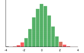
A confidence interval is a range of values that we believe the true population mean will fall between. In the example above, we have a 95% confidence interval when given a sample mean of 0, sample standard deviation of 10 and a sample size of 100. The graphic shows this sampling distribution and how only 5% of the samples would fall outside of the (-2, 2) range. Hence, we can be 95% confident that the true population mean is somewhere between -2 and 2.
Interpretation
On the AP exam, you are typically asked to create and interpret a confidence interval. 🔨
When asked to do this for a population mean, interpret your interval using the following template:
"I am % confident that the true population mean of ______________ is between (, ___)."
Rubrics generally include the following three aspects:
- Confidence level
- Context of problem
- Demonstrates knowledge that we are inferring about the true population mean 🎥 Watch: AP Stats - Inference: Confidence Intervals for Means
Vocabulary
The following words are mentioned explicitly in the College Board Course and Exam Description for this topic.Term | Definition |
|---|---|
confidence interval | A range of values, calculated from sample data, that is likely to contain the true population parameter with a specified level of confidence. |
confidence interval procedure | A statistical method used to construct an interval estimate for a population parameter based on sample data. |
critical value | A value from the standard normal distribution used to determine the margin of error for a given confidence level. |
degrees of freedom | A parameter of the t-distribution that affects its shape; as degrees of freedom increase, the t-distribution approaches the normal distribution. |
density curve | A graphical representation of a probability distribution showing the relative likelihood of different values. |
independence | The condition that observations in a sample are not influenced by each other, typically ensured through random sampling or randomized experiments. |
margin of error | The amount by which a sample statistic is likely to vary from the corresponding population parameter, calculated as the critical value times the standard error. |
matched pairs | Paired observations where two measurements are taken on the same subject or on subjects that are matched according to specific criteria, used to analyze the mean difference between the paired values. |
mean difference | The average of the differences between paired observations, denoted by μd, where the order of subtraction must be clearly defined. |
normal distribution | A probability distribution that is mound-shaped and symmetric, characterized by a population mean (μ) and population standard deviation (σ). |
one-sample t-interval | A confidence interval for a population mean constructed using the t-distribution when the population standard deviation is unknown. |
outlier | Data points that are unusually small or large relative to the rest of the data. |
population mean | The average of all values in an entire population, denoted as μ. |
population means | The average values of two distinct populations being compared, denoted as μ₁ and μ₂. |
population standard deviation | A measure of the spread or dispersion of all values in a population, denoted by σ, which is a parameter of the normal distribution. |
random sample | A sample selected from a population in such a way that every member has an equal chance of being chosen, reducing bias and allowing for valid statistical inference. |
randomized experiment | A study design where subjects are randomly assigned to treatment groups to establish cause-and-effect relationships. |
sample mean | The average of all values in a sample, denoted as x̄, used as an estimate of the population mean. |
sample size | The number of observations or data points collected in a sample, denoted as n. |
sample standard deviation | The standard deviation calculated for a sample, denoted by s, using the formula s = √(1/(n-1) ∑(xᵢ-x̄)²). |
sample statistic | A numerical value calculated from sample data that is used to estimate the corresponding population parameter. |
sampling distribution | The probability distribution of a sample statistic (such as a sample proportion) obtained from repeated sampling of a population. |
sampling without replacement | A sampling method in which an item selected from a population cannot be selected again in subsequent draws. |
skewness | A measure of the asymmetry of a distribution, indicating whether data is concentrated more on one side of the center. |
standard error | The standard deviation of a sampling distribution, which measures the variability of a sample statistic across repeated samples. |
t-distribution | A probability distribution used when the population standard deviation is unknown and the sample standard deviation is used instead, characterized by heavier tails than the normal distribution. |
tails | The extreme regions at both ends of a probability distribution's density curve where the t-distribution allocates more area than the normal distribution. |
Frequently Asked Questions
How do I know when to use a t-distribution instead of a normal distribution for confidence intervals?
Use a t-distribution whenever you don’t know the population standard deviation σ and must use the sample standard deviation s in your CI or test. The test statistic t = (x̄ − μ)/(s/√n) follows a t-distribution with df = n−1 (or for matched-pairs use npaired−1). Key checks from the CED before using a one-sample t-interval: - Independence: random sample or randomized experiment; if sampling without replacement, n ≤ 10% of N. - Normality of the sampling distribution of x̄: if sample size n > 30, the CLT usually makes x̄ approximately normal; if n ≤ 30, the sample data should show no strong skewness or outliers. Remember t-curves have thicker tails (more area in the tails) than the normal; as df increases t* approaches z*. Find t* from a t-table or computer output and use SE = s/√n so CI = x̄ ± t*(s/√n). For a quick review, see Fiveable’s Topic 7.2 study guide (https://library.fiveable.me/ap-statistics/unit-7/constructing-confidence-interval-for-population-mean/study-guide/Ol5pg6f4PKWs3n8reIZ5) and more unit resources (https://library.fiveable.me/ap-statistics/unit-7). For lots of practice, try the AP practice problems (https://library.fiveable.me/practice/ap-statistics).
What's the formula for a one-sample t-interval for a mean?
The one-sample t-interval for a population mean (σ unknown) is: x̄ ± t* · (s / √n) where x̄ = sample mean (point estimate), s = sample standard deviation, n = sample size, and t* is the critical t-value with df = n − 1 for your chosen confidence level. The margin of error = t*(s/√n). Before using it, check AP CED conditions: data are independent (random sample or randomized experiment; if sampling without replacement, n ≤ 10% of the population) and the sampling distribution of x̄ is approximately normal (either the original data are roughly symmetric/no strong outliers if n < 30, or n > 30 by CLT). t* values come from a t-table or computer output (df = n − 1). Note: the AP formula sheet gives standard error forms but not interval formulas, so you can build this from the general test-statistic and SE rules (see the Topic 7.2 study guide on Fiveable for more practice) (https://library.fiveable.me/ap-statistics/unit-7/constructing-confidence-interval-for-population-mean/study-guide/Ol5pg6f4PKWs3n8reIZ5). For more unit review and thousands of practice questions, check (https://library.fiveable.me/ap-statistics/unit-7) and (https://library.fiveable.me/practice/ap-statistics).
I'm confused about degrees of freedom - how do I calculate n-1 for t-distributions?
You just use n − 1 literally: if your sample has n observations, the one-sample t statistic t = (x̄ − μ) / (s/√n) has df = n − 1 (CED UNC-4.O.2). Why subtract 1? Because estimating the sample mean x̄ from the data “uses up” one piece of information (one parameter), so only n − 1 independent pieces remain to estimate variability (that’s what degrees of freedom mean here). Example: n = 10 → df = 9; n = 25 → df = 24. For matched pairs, treat the differences as one sample of size m (number of pairs) so df = m − 1. Larger df makes the t-distribution closer to normal (CED VAR-7.A.2). On the AP exam you’ll find t* values from the t-table (Formula Sheet/Table B) using df = n − 1. For a quick refresher, see the Topic 7.2 study guide on Fiveable (https://library.fiveable.me/ap-statistics/unit-7/constructing-confidence-interval-for-population-mean/study-guide/Ol5pg6f4PKWs3n8reIZ5) and try practice problems at (https://library.fiveable.me/practice/ap-statistics).
When do I need to check the 10% condition and what does n ≤ 10% N even mean?
Check the 10% condition anytime you sample without replacement from a finite population. The CED lists this under the independence check for inference: when you don’t replace items, you must verify n ≤ 10%·N to treat sample observations as (approximately) independent. Here n = your sample size and N = the total population size. Interpretation: n ≤ 0.10·N means your sample is at most 10% of the whole population (e.g., if N = 1,000 then n should be ≤ 100). If that holds, the dependence introduced by not replacing is negligible and the usual SE = s/√n (and t procedures) are valid. If n > 10%·N, independence is violated and you can’t use the standard formulas unless the study design (randomization, cluster sampling, etc.) justifies it or you apply a finite-population correction. For AP exam framing, always state you checked independence (random sampling or experiment) and the 10% condition when appropriate. For extra practice, see the Topic 7.2 study guide on Fiveable (https://library.fiveable.me/ap-statistics/unit-7/constructing-confidence-interval-for-population-mean/study-guide/Ol5pg6f4PKWs3n8reIZ5) and more practice problems at (https://library.fiveable.me/practice/ap-statistics).
What's the difference between standard error and margin of error in confidence intervals?
Standard error (SE) is the estimated standard deviation of your sample mean’s sampling distribution—for a one-sample t-interval SE = s/√n (CED UNC-4.Q.2). It measures how much x̄ would vary from sample to sample. Margin of error (ME) is how far you go above and below the point estimate to make a confidence interval: ME = (critical value) × SE. For a t-interval that’s ME = t*·(s/√n) (CED UNC-4.Q.3, UNC-4.R.2). So SE is about variability of the estimator; ME turns that variability into a confidence “buffer” using the t* that depends on your confidence level and df (CED VAR-7.A). Remember to check independence and approximate normality before using t-intervals (CED UNC-4.P). For a quick refresher, see the Topic 7.2 study guide (https://library.fiveable.me/ap-statistics/unit-7/constructing-confidence-interval-for-population-mean/study-guide/Ol5pg6f4PKWs3n8reIZ5) and practice problems (https://library.fiveable.me/practice/ap-statistics).
How do I find the critical value t* on my calculator for a 95% confidence interval?
You need the t* that leaves (1–CL)/2 in each tail. Find it with your calculator using the inverse t (quantile) function and df = n–1. For a 95% CI CL = 0.95 so use 0.975 as the cumulative probability. - TI-84/TI-83: 2nd → DISTR → invT(0.975, df). - TI-Nspire: Menu → Statistics → Distributions → Student’s t inverse → P = 0.975, df = n–1. - If you only have a t-table, look under 0.025 tail (two-tailed 95%) for df = n–1 and read t*. Remember: this is for a one-sample t-interval (σ unknown) and df = n–1 (CED UNC-4.O.2, UNC-4.Q.1). Before using the t-interval check independence and approximate normality (CED UNC-4.P). For a refresher see the Topic 7.2 study guide (https://library.fiveable.me/ap-statistics/unit-7/constructing-confidence-interval-for-population-mean/study-guide/Ol5pg6f4PKWs3n8reIZ5) and more practice problems (https://library.fiveable.me/practice/ap-statistics).
Can someone explain step by step how to construct a confidence interval for a population mean?
Step-by-step: one-sample t-interval for a mean 1. Check conditions (UNC-4.P): data are from a random sample or randomized experiment (independence), and n ≤ 10% of the population if sampling without replacement. Check sampling distribution is approx. normal: if n>30 CLT helps; if n≤30, the sample data should have no strong skewness or outliers. 2. Compute the point estimate: sample mean x̄. 3. Compute the standard error (UNC-4.Q.2): SE = s/√n, where s is the sample standard deviation. 4. Find degrees of freedom: df = n − 1. Look up the critical t* for your confidence level and df (table or calculator) (UNC-4.Q.1). 5. Margin of error (UNC-4.Q.3): ME = t* × SE. 6. Confidence interval (UNC-4.R.2): x̄ ± ME. 7. Interpret in context: “We are [C]% confident the population mean [context] lies between ___ and ___.” For matched pairs, form differences first and treat as one sample of differences. For extra practice and AP-aligned help, see the Topic 7.2 study guide (https://library.fiveable.me/ap-statistics/unit-7/constructing-confidence-interval-for-population-mean/study-guide/Ol5pg6f4PKWs3n8reIZ5) and tons of practice problems (https://library.fiveable.me/practice/ap-statistics).
I don't understand when the sample size needs to be greater than 30 vs less than 30 - what's the rule?
Short answer: the cutoff isn't magic—it's about the sampling distribution being approximately normal. Use a one-sample t-interval whenever σ is unknown (almost always). Then check conditions: - Independence (random sample or experiment; if sampling without replacement, n ≤ 10% of N). - Normality of the sampling distribution of x̄ (shape): - If n ≥ 30, the CLT usually makes x̄ ≈ normal even with moderate skew, so the t-interval is safe. - If n < 30, you need the sample data (or population) to be close to normal—no strong skewness or outliers—for the t-interval to be valid. Also remember degrees of freedom = n − 1 and SE = s/√n; margin of error = t*·(s/√n). On the AP exam you should verify independence and normality in context (compare p-value/CI logic), and you can build formulas from the general test-statistic form (they’re not given on the formula sheet). For more review see Fiveable’s Topic 7.2 study guide (https://library.fiveable.me/ap-statistics/unit-7/constructing-confidence-interval-for-population-mean/study-guide/Ol5pg6f4PKWs3n8reIZ5), the unit overview (https://library.fiveable.me/ap-statistics/unit-7), and extra practice (https://library.fiveable.me/practice/ap-statistics).
What conditions do I need to check before making a t-interval and how do I write them on the FRQ?
Before you write a t-interval on an FRQ, check two things: independence and normality of the sampling distribution. - Independence: state that the data come from a random sample or randomized experiment. If sampling without replacement, say n ≤ 10% of the population (10% condition). - Normality (shape): if n > 30 you can usually rely on the CLT; if n ≤ 30 you must say the sample distribution shows no strong skewness or outliers (use a histogram/boxplot or describe skewness). For matched pairs, apply these checks to the paired differences. How to write it on the FRQ (short, AP style): - “Conditions: Data are from a random sample/experiment, so observations are independent. n = ___ ≤ 10% of the population, so 10% condition met.” - “Sampling distribution: n = ___ (>30) so CLT applies / OR n = ___ (≤30) and the sample histogram/boxplot of x (or differences) is roughly symmetric with no outliers, so approximate normality holds.” - Then conclude: “Therefore a one-sample t-interval is appropriate.” For more review and examples see the Topic 7.2 study guide (https://library.fiveable.me/ap-statistics/unit-7/constructing-confidence-interval-for-population-mean/study-guide/Ol5pg6f4PKWs3n8reIZ5) and unit resources (https://library.fiveable.me/ap-statistics/unit-7). For practice, try problems at https://library.fiveable.me/practice/ap-statistics.
How do I solve a matched pairs confidence interval problem?
Think of matched pairs as one sample of differences. Steps to do a matched-pairs CI for the mean difference (d = before − after or paired1 − paired2): 1. Compute differences di for each pair. Get x̄d and sd (sample mean and SD of the differences). n = number of pairs. 2. Verify conditions (CED UNC-4.P): data collected randomly, n ≤ 10% of population if sampling without replacement, and the sampling distribution of x̄d is approximately normal (if n<30 check the distribution of the di’s for strong skewness/outliers). 3. Use a one-sample t-interval with df = n−1: SE = sd/√n. Find t* for your confidence level and df (CED UNC-4.Q). 4. Margin of error = t*·SE. CI: x̄d ± t*·SE. Interpret in context (e.g., “We are [CL]% confident the mean (before−after) difference is between …”). Remember the AP note: you can build this formula from the general test statistic and SE on the formula sheet. For more examples and practice, see the Topic 7.2 study guide (https://library.fiveable.me/ap-statistics/unit-7/constructing-confidence-interval-for-population-mean/study-guide/Ol5pg6f4PKWs3n8reIZ5) and unit practice (https://library.fiveable.me/practice/ap-statistics).
Why does the t-distribution have more area in the tails than a normal distribution?
Because we replace the unknown population σ with the sample s, the standardized statistic t = (x̄ − μ)/(s/√n) has extra randomness. s itself varies from sample to sample, especially when n is small (degrees of freedom = n − 1). That extra variability makes extreme values of t more likely than extreme z values, so the t-density puts more area in the tails. As n (and thus df) increases, s becomes a more stable estimate of σ, the extra variability shrinks, and the t-distribution approaches the Normal—so tail area decreases with higher df (VAR-7.A.1 and VAR-7.A.2 in the CED). On the AP exam you use a t* critical value that depends on df (see the t-table on the formula sheets), which makes margins of error larger for small samples. For a quick refresher, check the Topic 7.2 study guide (https://library.fiveable.me/ap-statistics/unit-7/constructing-confidence-interval-for-population-mean/study-guide/Ol5pg6f4PKWs3n8reIZ5) and try practice problems at (https://library.fiveable.me/practice/ap-statistics).
What happens to the t-distribution as degrees of freedom increase?
Short answer: as degrees of freedom (df) increase, the t-distribution’s tails get less heavy and the curve approaches the standard normal. With small df the t has more area in the tails (wider spread) because s is a noisier estimate of σ; as df grows (for a one-sample t, df = n − 1) that noise shrinks, so the t critical values t* move closer to the z critical values. Practically: small samples → bigger t* → larger margin of error (t*(s/√n)); large samples (say df ≥ 30–40) → t* ≈ z and the t-interval behaves like a z-interval. On the AP exam you’ll find t* using the provided t-table or your calculator (CED UNC-4.Q.1, VAR-7.A.2); review Topic 7.2 on Fiveable for examples and practice (https://library.fiveable.me/ap-statistics/unit-7/constructing-confidence-interval-for-population-mean/study-guide/Ol5pg6f4PKWs3n8reIZ5).
I keep getting the wrong margin of error - is it t* times s over square root of n?
Yes—for a one-sample t-interval the margin of error (ME) is t* × SE and SE = s/√n, so ME = t*(s/√n). Use t* from the t-distribution with df = n − 1 for your chosen confidence level (table or calculator). Make sure the conditions from the CED are met before using this: independence (random sample or randomized experiment and n ≤ 10% of population if sampling without replacement) and an approximately normal sampling distribution (if n < 30 check the data for strong skewness/outliers; larger n lets CLT help). As the CED notes, t-distributions have heavier tails and t* depends on df (use Table B or your calculator). The AP exam gives tables but not interval formulas, so you should be able to build the interval as x̄ ± t*(s/√n). For a quick topic review see the Fiveable study guide (https://library.fiveable.me/ap-statistics/unit-7/constructing-confidence-interval-for-population-mean/study-guide/Ol5pg6f4PKWs3n8reIZ5) and try practice problems (https://library.fiveable.me/practice/ap-statistics).
How do I know if my data is too skewed to use a t-interval when n is small?
If n is small (CED rule: n < 30), you must check the sample distribution for strong skewness or outliers before using a one-sample t-interval. Practically: - Make a histogram or boxplot. If the shape is roughly symmetric and there are no extreme outliers, a t-interval is OK. - If you see clear right/left skew or big outliers, the t-interval may be invalid for small n (CED: “distribution should be free from strong skewness and outliers” when n < 30). - Also verify independence (random sample or experiment and n ≤ 10% of population if no replacement). If the sample is too skewed, use a transformation (log, etc.), a nonparametric method, or a bootstrap CI instead. For AP practice and walkthroughs on checking conditions, see the Topic 7.2 study guide (https://library.fiveable.me/ap-statistics/unit-7/constructing-confidence-interval-for-population-mean/study-guide/Ol5pg6f4PKWs3n8reIZ5) and Unit 7 review (https://library.fiveable.me/ap-statistics/unit-7). For extra practice, try problems at (https://library.fiveable.me/practice/ap-statistics).
What's the point estimate for a population mean and how is it different from the confidence interval?
The point estimate for a population mean is the sample mean x̄—it’s your best single-number guess for μ (CED: UNC-4.R.1). A confidence interval, by contrast, gives a range of plausible values for μ built around that point estimate: x̄ ± t*(s/√n). Here s/√n is the standard error, t* is the critical t with n−1 degrees of freedom, and the margin of error = t*(s/√n) (CED: UNC-4.Q, UNC-4.R). So: x̄ is one number; the CI is that number plus/minus a margin that reflects sampling variability and your chosen confidence level. Remember to verify conditions before trusting the interval: random/independent data (10% rule), and an approximately normal sampling distribution (n>30 or no strong skew/outliers for small n)—use the t-distribution when σ is unknown (CED: UNC-4.P, VAR-7.A). For more practice and a topic review see the Topic 7.2 study guide (https://library.fiveable.me/ap-statistics/unit-7/constructing-confidence-interval-for-population-mean/study-guide/Ol5pg6f4PKWs3n8reIZ5) and unit resources (https://library.fiveable.me/ap-statistics/unit-7).