Differences (Non-Distribution) Recap
To find the sampling distribution for differences in a sample proportion or mean, remember that variances always add to find the new variance. If one needs the standard deviation, you should take the square root of the variance. However, for means you can just subtract.

Proportion Differences
To find the standard deviation of differences in sample means, divide the variances by each sample size before square rooting to find the overall standard deviation. The simplified formula can be seen below. If you are only given the standard deviations for both samples, you must square both standard deviations, add them up and then take the square root. This can be referred to as the “**Pythagorean Theorem of Statistics.” **
For any Proportion Inference, you must check Large Counts to confirm normality. You can only check Central Limit Theorem for Quantitative Data (Means).
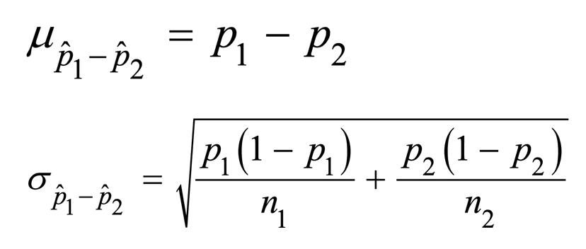
For a categorical variable, when randomly sampling with replacement from two independent populations with population proportions p1 and p2, the sampling distribution of the difference in sample proportions, p1 - p2, has mean µ = p1 - p2 and standard deviation as shown in the image below.
Additionally, the sampling distribution of the difference in sample proportions p1 - p2 will have an approximate normal distribution provided the sample sizes are large enough:
- n1p1 > 10
- n1 (1 - p1) > 10
- n2p2 > 10
- n2 (1 - p2) > 10
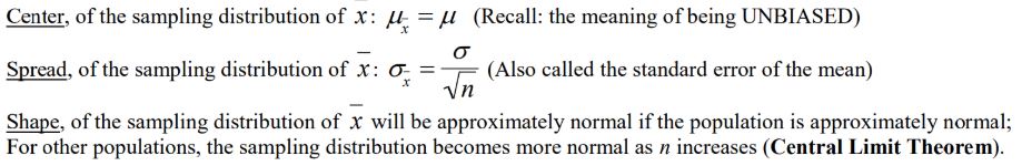
Here is a review of types of distributions: (Be sure to save this somewhere!)

Practice Problem
Suppose that you are conducting a survey to compare the proportion of people in two different cities who support a new public transportation system. You decide to use simple random samples of 1000 people from each city, and you ask them whether or not they support the new system. After collecting the data, you find that 600 people out of the 1000 respondents from City A support the system, and 700 people out of the 1000 respondents from City B support the system.
a) Calculate the sample proportions of respondents who support the new system in each city.
b) Explain what the sampling distribution for the difference in sample proportions represents and why it is useful in this situation.
c) Suppose that the true population proportion of people in City A who support the new system is actually 0.6, and the true population proportion of people in City B who support the new system is actually 0.7. Describe the shape, center, and spread of the sampling distribution for the difference in sample proportions in this case.
d) Explain why the Central Limit Theorem applies to the sampling distribution for the difference in sample proportions in this situation.
e) Discuss one potential source of bias that could affect the results of this study, and explain how it could influence the estimate. (Hint: slightly different when thinking about working with one sample vs. two samples)
Answer
a) The sample proportion of respondents who support the new system in City A is 600/1000 = 0.6, and the sample proportion of respondents who support the new system in City B is 700/1000 = 0.7.
b) The sampling distribution for the difference in sample proportions represents the distribution of possible values for the difference between the sample proportions if the study were repeated many times. It is useful in this situation because it allows us to make inferences about the difference between the population proportions in the two cities based on the sample data.
c) If the true population proportion of people in City A who support the new system is 0.6, and the true population proportion of people in City B who support the new system is 0.7, the sampling distribution for the difference in sample proportions would be approximately normal with a center at 0.7 - 0.6 = 0.1 and a spread that depends on the sample sizes and the variability of the populations.
d) The Central Limit Theorem applies to the sampling distribution for the difference in sample proportions in this situation because the sample sizes (n1 = 1000 and n2 = 1000) are large enough for the distribution to be approximately normal, even if the populations are not normally distributed.
e) One potential source of bias in this study could be nonresponse bias, which occurs when certain groups of individuals are more or less likely to respond to the survey. For example, if people in City A who support the new system are more likely to respond to the survey, the sample from City A could be biased toward higher levels of support and produce an overestimate of the population proportion.
On the other hand, if people in City B who do not support the new system are more likely to respond, the sample from City B could be biased toward lower levels of support and produce an underestimate of the population proportion. This could lead to an incorrect estimate of the difference in population proportions between the two cities.
Vocabulary
The following words are mentioned explicitly in the College Board Course and Exam Description for this topic.
| Term | Definition |
|---|---|
| approximately normal | A distribution that closely follows the shape of a normal distribution, allowing for the use of normal probability methods. |
| categorical variable | A variable that takes on values that are category names or group labels rather than numerical values. |
| difference in proportions | The difference between two population proportions, calculated as p₁ - p₂, used to compare the prevalence of a characteristic across two populations. |
| difference in sample proportions | The difference between two sample proportions (p̂₁ - p̂₂) used to compare proportions from two different samples. |
| independent populations | Two populations from which samples are drawn such that the selection from one population does not affect the selection from the other. |
| mean of the sampling distribution | The expected value of a sample statistic; for sample proportions, μp̂ = p. |
| normality conditions | The requirements that must be met for a sampling distribution to be approximately normal, such as n₁p₁ ≥ 10, n₁(1-p₁) ≥ 10, n₂p₂ ≥ 10, and n₂(1-p₂) ≥ 10. |
| parameter | A numerical summary that describes a characteristic of an entire population. |
| population proportion | The true proportion or percentage of a characteristic in an entire population, typically denoted as p. |
| probability | The likelihood or chance that a particular outcome or event will occur, expressed as a value between 0 and 1. |
| sample proportion | The proportion of individuals in a sample that have a particular characteristic, denoted as p-hat (p̂). |
| sample size | The number of observations or data points collected in a sample, denoted as n. |
| sampling distribution | The probability distribution of a sample statistic (such as a sample proportion) obtained from repeated sampling of a population. |
| sampling with replacement | A sampling method in which an item selected from a population can be selected again in subsequent draws. |
| sampling without replacement | A sampling method in which an item selected from a population cannot be selected again in subsequent draws. |
| standard deviation of the sampling distribution | The measure of variability in a sampling distribution; for sample proportions, σp̂ = √(p(1-p)/n). |
Frequently Asked Questions
What's the formula for the standard deviation of the difference in sample proportions?
If you have two independent random samples with population proportions p1 and p2 and sample sizes n1 and n2, the sampling distribution of p̂1 − p̂2 has mean μ = p1 − p2 and standard deviation σ(p̂1 − p̂2) = sqrt[ p1(1 − p1)/n1 + p2(1 − p2)/n2 ]. In practice when doing inference you usually estimate that with sample proportions: SE = sqrt[ p̂1(1 − p̂1)/n1 + p̂2(1 − p̂2)/n2 ]. If you’re running a two-sample z-test and you assume p1 = p2 under H0, use the pooled proportion p̂c = (X1+X2)/(n1+n2) and SE = sqrt[ p̂c(1−p̂c)(1/n1 + 1/n2) ]. If sampling without replacement and n is ≥10% of the population, use the finite-population correction (it makes σ smaller). Also check success–failure conditions (n1p1, n1(1−p1), n2p2, n2(1−p2) ≥ 10) before using the normal approximation. More review on Topic 5.6 here (https://library.fiveable.me/ap-statistics/unit-5/sampling-distributions-for-differences-sample-proportions/study-guide/VOvA8du6YHMjhEwB7lEW) and practice problems at (https://library.fiveable.me/practice/ap-statistics).
How do I know when to use the sampling distribution for difference in proportions vs just regular proportion?
Use the difference-in-proportions model when you’re comparing two independent groups (two samples) and your statistic is p̂1 − p̂2. Use a single-proportion model when you have only one sample and your statistic is p̂. Key checks for the two-proportion sampling distribution (CED UNC-3.N/O/P): - Samples must be independent random samples (or <10% of each population if not replaced). - Success–failure: n1p1 ≥ 10, n1(1−p1) ≥ 10, n2p2 ≥ 10, n2(1−p2) ≥ 10 for approximate normality. - Mean of p̂1 − p̂2 = p1 − p2; SD = sqrt[ p1(1−p1)/n1 + p2(1−p2)/n2 ] (use p̂’s for SE in practice). For hypothesis tests when H0: p1 = p2, use the pooled proportion p̂c for the SE. For one-sample inference about a single population proportion, use the one-sample formula and success–failure for that sample only. For a quick review see the Topic 5.6 study guide (https://library.fiveable.me/ap-statistics/unit-5/sampling-distributions-for-differences-sample-proportions/study-guide/VOvA8du6YHMjhEwB7lEW) and more practice at the Unit 5 page (https://library.fiveable.me/ap-statistics/unit-5) or practice problems (https://library.fiveable.me/practice/ap-statistics).
Can someone explain step by step how to find the mean and standard deviation for p̂₁ - p̂₂?
Step-by-step: mean and SD for p̂1 − p̂2 1. Identify population proportions p1 and p2 and sample sizes n1 and n2 (from two independent random samples). 2. Mean (expected value) of the sampling distribution: μ(p̂1 − p̂2) = p1 − p2. This is just the difference of the population proportions (CED UNC-3.N.1). 3. Standard deviation (standard error) when sampling with replacement or when samples <10% of populations: σ(p̂1 − p̂2) = sqrt[ p1(1 − p1)/n1 + p2(1 − p2)/n2 ]. Plug in p1, p2, n1, n2, compute each fraction, add, then take the square root. 4. Check normal approx (for inference): n1 p1 ≥ 10, n1(1−p1) ≥ 10, n2 p2 ≥ 10, n2(1−p2) ≥ 10 (CED UNC-3.O.1). If these hold, p̂1 − p̂2 ≈ Normal. 5. For hypothesis tests that assume p1 = p2 under H0, use the pooled proportion p̂c = (X1+X2)/(n1+n2) to compute the SE: sqrt[ p̂c(1−p̂c)(1/n1 + 1/n2) ]. For a clear walkthrough and examples, see the Topic 5.6 study guide (https://library.fiveable.me/ap-statistics/unit-5/sampling-distributions-for-differences-sample-proportions/study-guide/VOvA8du6YHMjhEwB7lEW) and more practice at the Unit 5 page (https://library.fiveable.me/ap-statistics/unit-5) or the practice problem bank (https://library.fiveable.me/practice/ap-statistics).
When do I use the 10% rule for sampling without replacement and how does it affect my calculations?
Use the 10% rule whenever you sample without replacement from a finite population. It’s a quick check for independence: if your sample size n is less than 10% of the population N (n < 0.10N), you can treat draws as (practically) independent and use the usual SE formulas. If n ≥ 0.10N, independence is violated enough that you should apply the finite population correction (FPC), which makes the standard errors smaller. For two proportions, include the FPC for each sample: SE(p̂1 − p̂2) = sqrt[ p1(1−p1)/n1 * ((N1−n1)/(N1−1)) + p2(1−p2)/n2 * ((N2−n2)/(N2−1)) ]. If n1 and n2 are both < 10% of N1 and N2 you can drop the FPCs and use the CED formula σ = sqrt(p1(1−p1)/n1 + p2(1−p2)/n2). Don’t forget AP exam checks: also verify success–failure (n p ≥ 10 and n(1−p) ≥ 10) before using the normal approximation. For a focused walkthrough see the Topic 5.6 study guide (https://library.fiveable.me/ap-statistics/unit-5/sampling-distributions-for-differences-sample-proportions/study-guide/VOvA8du6YHMjhEwB7lEW). For broader review and practice, use the Unit 5 page (https://library.fiveable.me/ap-statistics/unit-5) and practice problems (https://library.fiveable.me/practice/ap-statistics).
What are the conditions I need to check before I can say the sampling distribution is approximately normal?
You need to check three things before you can say p̂1 − p̂2 is approximately normal (per the CED): 1. Independent random samples (or randomized experiment) from two populations—and if sampling without replacement, each sample size < 10% of its population (the 10% condition). 2. Success–failure condition for both samples: n1·p1 ≥ 10, n1·(1−p1) ≥ 10, n2·p2 ≥ 10, n2·(1−p2) ≥ 10. (If you don’t know p1,p2 for planning, use expected or sample proportions.) 3. Two samples are independent of each other (different subjects/groups). If these hold, the sampling distribution has mean μ(p̂1−p̂2)=p1−p2 and SE = sqrt[p1(1−p1)/n1 + p2(1−p2)/n2] and you can use the normal approximation for CIs or two-sample z-tests (what AP expects in Topic 5.6). For more examples and a focused study guide, see the Topic 5.6 study guide (https://library.fiveable.me/ap-statistics/unit-5/sampling-distributions-for-differences-sample-proportions/study-guide/VOvA8du6YHMjhEwB7lEW). Practice lots of problems at (https://library.fiveable.me/practice/ap-statistics).
I'm confused about why we subtract the proportions - when would I actually need to find p̂₁ - p̂₂ in a real problem?
You subtract proportions when you’re comparing two groups—p̂1 − p̂2 is the difference in sample proportions and answers questions like “Is the vaccination rate higher in City A than City B?” or “Did the proportion of students preferring option X change between two years?” The sampling distribution has mean μ(p̂1−p̂2)=p1−p2 and SE = sqrt[p1(1−p1)/n1 + p2(1−p2)/n2]; for inference use a two-sample z-test or a CI for p1−p2. Check success–failure: n1p1, n1(1−p1), n2p2, n2(1−p2) ≥ 10 (or use p̂s for practical checking). If you assume p1 = p2 for a hypothesis test, use the pooled proportion p̂c in the SE. These ideas show up on the AP exam (Unit 5 & Unit 6 inference topics)—review Topic 5.6 on Fiveable (https://library.fiveable.me/ap-statistics/unit-5/sampling-distributions-for-differences-sample-proportions/study-guide/VOvA8du6YHMjhEwB7lEW), the Unit 5 overview (https://library.fiveable.me/ap-statistics/unit-5), and grab practice problems at (https://library.fiveable.me/practice/ap-statistics) to solidify this.
How do I solve problems where they give me two different sample sizes and ask for the probability that one proportion is bigger than the other?
Use the sampling distribution for p̂1 − p̂2 and the Normal approx. Steps: 1. Identify p1 and p2 (use population proportions if given; if only sample results are given, use p̂1 and p̂2 as estimates). 2. Check success–failure: n1 p1 ≥ 10, n1(1−p1) ≥ 10, n2 p2 ≥ 10, n2(1−p2) ≥ 10 (if using sample props, check with p̂s). If sampling without replacement, make sure n < 0.10N or ignore FPC. 3. Mean = μ = p1 − p2. Standard error = σ = sqrt[ p1(1−p1)/n1 + p2(1−p2)/n2 ]. If you only have sample counts and you’re doing a test of p1 = p2, use the pooled p̂c for the SE: sqrt[p̂c(1−p̂c)(1/n1+1/n2)]. 4. To get P(p̂1 > p̂2) compute P(p̂1 − p̂2 > 0). Standardize: Z = (0 − μ)/σ, then find P(Z > (0−μ)/σ) = 1 − Φ((0−μ)/σ) (or use Φ with sign). Example quick: if p1=0.6, p2=0.5, n1=100, n2=200 → μ=0.1, σ= sqrt(0.6·0.4/100 + 0.5·0.5/200)=... then Z=(0−0.1)/σ and P = 1−Φ(Z). For more detail and examples, see the Topic 5.6 study guide (https://library.fiveable.me/ap-statistics/unit-5/sampling-distributions-for-differences-sample-proportions/study-guide/VOvA8du6YHMjhEwB7lEW). Practice problems are at (https://library.fiveable.me/practice/ap-statistics).
What's the difference between the sampling distribution for one proportion and the sampling distribution for difference in proportions?
Short answer: the sampling distribution for one sample proportion p̂ has mean μp̂ = p and standard error σp̂ = √[p(1−p)/n]. For the difference of two independent sample proportions p̂1 − p̂2, the sampling distribution has mean μ = p1 − p2 and standard error σ = √[p1(1−p1)/n1 + p2(1−p2)/n2] (CED UNC-3.N.1). Important practical differences you’ll use on the AP exam: - Condition for approximate normality for one proportion: np ≥ 10 and n(1−p) ≥ 10. For two proportions, check n1p1, n1(1−p1), n2p2, n2(1−p2) ≥ 10 (CED UNC-3.O.1). - For hypothesis tests where p1 = p2 is assumed, use the pooled proportion p̂c for the standard error. - If sampling without replacement and sample >10% of population, apply the finite-population correction (otherwise negligible) (CED UNC-3.N.2). Want more examples and practice? See the Topic 5.6 study guide (https://library.fiveable.me/ap-statistics/unit-5/sampling-distributions-for-differences-sample-proportions/study-guide/VOvA8du6YHMjhEwB7lEW) and hit the AP practice bank (https://library.fiveable.me/practice/ap-statistics).
Do I need to check n₁p₁ ≥ 10 AND n₁(1-p₁) ≥ 10 for BOTH samples or just one?
You need to check the success–failure condition for both samples. The CED’s rule (UNC-3.O.1) requires n1p1 ≥ 10 and n1(1−p1) ≥ 10 AND n2p2 ≥ 10 and n2(1−p2) ≥ 10 so the sampling distribution of p̂1 − p̂2 is approximately normal. A practical note for inference: if you’re doing a two-sample z-test and the null assumes p1 = p2, you use the pooled proportion p̂c to check the condition (n1 p̂c ≥ 10, n1(1−p̂c) ≥ 10, etc.). If you’re building a CI or not pooling, check each sample with its own p̂. If sampling without replacement, make sure each sample is <10% of its population (finite-pop correction negligible otherwise). For more AP-aligned explanation and examples, see the Topic 5.6 study guide (https://library.fiveable.me/ap-statistics/unit-5/sampling-distributions-for-differences-sample-proportions/study-guide/VOvA8du6YHMjhEwB7lEW) and try practice problems (https://library.fiveable.me/practice/ap-statistics).
I don't understand why the standard deviation formula has that square root with both fractions added together - can someone break this down?
Think of p̂1 and p̂2 as two independent random variables. The standard deviation of their difference comes from variance rules: for independent variables, Var(A − B) = Var(A) + Var(B). Each sample proportion has Var(p̂) = p(1 − p)/n, so Var(p̂1 − p̂2) = p1(1−p1)/n1 + p2(1−p2)/n2. The standard deviation is the square root of that variance, so σ(p̂1−p̂2) = √[p1(1−p1)/n1 + p2(1−p2)/n2]. The plus sign isn’t a mistake—variances add for independent sampling, even though you’re subtracting the statistics. Two quick reminders from the CED: this formula assumes independent random samples (or sampling with replacement); if you sample without replacement and n’s are >10% of populations, use the finite-population correction. Also check success–failure (n1p1, n1(1−p1), n2p2, n2(1−p2) ≥ 10) before using the normal approximation. For more AP-aligned review, see the Topic 5.6 study guide (https://library.fiveable.me/ap-statistics/unit-5/sampling-distributions-for-differences-sample-proportions/study-guide/VOvA8du6YHMjhEwB7lEW) and extra practice (https://library.fiveable.me/practice/ap-statistics).
How do I interpret what it means when they ask for P(p̂₁ - p̂₂ > 0.05) in context of the actual populations?
P(p̂1 − p̂2 > 0.05) asks: if you take one random sample from population 1 and one from population 2, what’s the probability the observed difference in sample proportions (p̂1 − p̂2) will be more than 0.05? In terms of the populations, it’s the chance that your samples produce an estimate at least 5 percentage points larger than the other—given the true population proportions p1 and p2, the sampling distribution of p̂1 − p̂2 has mean p1 − p2 and SE = sqrt[p1(1−p1)/n1 + p2(1−p2)/n2]. Using the normal approximation (check n1p1, n1(1−p1), n2p2, n2(1−p2) ≥ 10), convert 0.05 to a z-score and find the tail probability. Interpret the result as a long-run probability over many repeated independent samples (UNC-3.P.1). For a refresher, see the Topic 5.6 study guide (https://library.fiveable.me/ap-statistics/unit-5/sampling-distributions-for-differences-sample-proportions/study-guide/VOvA8du6YHMjhEwB7lEW) and try practice problems (https://library.fiveable.me/practice/ap-statistics).
What happens to my calculations if the sample sizes are more than 10% of the population sizes?
If your sample sizes are more than 10% of their populations, the usual SE formula for p̂1 − p̂2 (√[p1(1−p1)/n1 + p2(1−p2)/n2]) will overestimate the true variability because that formula assumes sampling with replacement (or effectively infinite populations). The CED notes this (UNC-3.N.2): when sampling without replacement and n is not <10% of N, apply the finite population correction (FPC). For one sample multiply its variance term by (N−n)/(N−1); for two independent samples apply each sample’s FPC separately. So the SE becomes: √[ p1(1−p1)/n1 · (N1−n1)/(N1−1) + p2(1−p2)/n2 · (N2−n2)/(N2−1) ]. The success–failure conditions and normal-approx rules (n p ≥ 10 and n(1−p) ≥ 10 for each sample) still apply for approximate normality (UNC-3.O.1). For worked examples and exam-style practice, check the Topic 5.6 study guide (https://library.fiveable.me/ap-statistics/unit-5/sampling-distributions-for-differences-sample-proportions/study-guide/VOvA8du6YHMjhEwB7lEW) and more practice problems (https://library.fiveable.me/practice/ap-statistics).
Can I use my calculator to find probabilities for sampling distributions of differences, and if so, what do I plug into normalcdf?
Yes—use your graphing calculator (TI-style) to get normal probabilities for p̂1 − p̂2 when the sampling distribution is approximately normal (check success–failure: n1p1 ≥10, n1(1−p1) ≥10, same for sample 2). Step 1: compute the distribution parameters from the CED: - mean = μ = p1 − p2 - standard deviation = σ = sqrt[ p1(1−p1)/n1 + p2(1−p2)/n2 ] Step 2: use normalcdf(lower, upper, mean, sd). Examples (TI-84 syntax): - P(p̂1 − p̂2 > 0.05) = normalcdf(0.05, 1E99, μ, σ) - P(−0.02 < p̂1 − p̂2 < 0.03) = normalcdf(−0.02, 0.03, μ, σ) - P(p̂1 − p̂2 ≤ 0) = normalcdf(−1E99, 0, μ, σ) On AP exam bring a permitted calculator and use these commands. For hypothesis tests that assume p1 = p2 (two-sample z-test), use the pooled proportion only when calculating the test SE—not when describing the sampling distribution under known p1,p2. For a concise review, see the Topic 5.6 study guide (https://library.fiveable.me/ap-statistics/unit-5/sampling-distributions-for-differences-sample-proportions/study-guide/VOvA8du6YHMjhEwB7lEW) and practice problems at (https://library.fiveable.me/practice/ap-statistics).
Step by step, how do I set up a problem that asks me to compare proportions from two different groups like men vs women or treatment vs control?
1) State parameter: p1 − p2 (e.g., proportion men − proportion women). 2) Collect data: find x1, n1, x2, n2 and compute p̂1 = x1/n1, p̂2 = x2/n2 and the difference p̂1 − p̂2. 3) Check independence and random sampling; if without replacement verify each sample <10% of its population. 4) Check normal approximation (success–failure): n1p1 ≥10, n1(1−p1) ≥10, n2p2 ≥10, n2(1−p2) ≥10. If true, p̂1 − p̂2 is approx normal (CED UNC-3.O.1). 5) Parameter of sampling distribution: μ(p̂1−p̂2)=p1−p2 and standard error: σ = sqrt[ p1(1−p1)/n1 + p2(1−p2)/n2 ]. For inference use estimated SE with p̂s: SE = sqrt[ p̂1(1−p̂1)/n1 + p̂2(1−p̂2)/n2 ]. 6) For a two-sample z test when H0: p1=p2, use pooled p̂c = (x1+x2)/(n1+n2) to compute SE = sqrt[ p̂c(1−p̂c)(1/n1+1/n2) ]. 7) Compute z = (p̂1−p̂2 − 0)/SE, find p-value, and interpret in context. Need examples or practice? See the Topic 5.6 study guide (https://library.fiveable.me/ap-statistics/unit-5/sampling-distributions-for-differences-sample-proportions/study-guide/VOvA8du6YHMjhEwB7lEW) and try problems at Fiveable practice (https://library.fiveable.me/practice/ap-statistics).