18.1 Time-domain analysis of continuous-time systems

Continuous-Time Signals and Systems

Signal and System Properties

A continuous-time signal is any signal defined for every value of time along a continuous range, written mathematically as $x(t)$. Think of a voltage measured across a resistor or the temperature in a room throughout the day. Unlike discrete-time signals (which only exist at specific time steps), these signals have a value at every instant.

The systems that process these signals have several important properties:

• Linearity means the system obeys superposition. If input $x_1(t)$ produces output $y_1(t)$ and input $x_2(t)$ produces output $y_2(t)$, then input $ax_1(t) + bx_2(t)$ produces output $ay_1(t) + by_2(t)$. You can scale and add inputs, and the outputs scale and add the same way.
• Time-invariance means the system's behavior doesn't change over time. If you delay the input by $t_0$ seconds, the output is simply delayed by the same $t_0$ seconds. The system treats a signal the same whether it arrives now or an hour from now.
• Causality means the output at any time $t$ depends only on the present and past values of the input, never on future values. Almost all physical systems are causal, since real hardware can't peek ahead in time.
• Stability (specifically, BIBO stability) means that every bounded input produces a bounded output. If you feed in a signal that stays finite, the output stays finite too. An unstable system can blow up to infinity even from a well-behaved input, which usually means something has gone wrong in your design.

A system that has both linearity and time-invariance is called a linear time-invariant (LTI) system. LTI systems are the focus of most introductory analysis because they're mathematically tractable and they model many real circuits and physical processes well.

System Characteristics and Behavior

Three tools form the backbone of time-domain analysis for LTI systems: the impulse response, the step response, and differential equations.

Impulse response $h(t)$ is the output you get when the input is a unit impulse $\delta(t)$. This single function completely describes an LTI system. Once you know $h(t)$, you can find the output for any input using convolution (covered below).

Step response is the output when the input is a unit step $u(t)$. Because the step function is the integral of the impulse, the step response is the integral of the impulse response. The step response is especially useful for evaluating how a system transitions from rest to a new steady state. Engineers extract several performance metrics from it:

• Rise time: how long the output takes to go from 10% to 90% of its final value.
• Settling time: how long until the output stays within a small band (typically 2%) of its final value.
• Overshoot: how far the output exceeds its final value before settling down.
• Steady-state value: the value the output approaches as $t \to \infty$.

Differential equations provide the mathematical model linking input $x(t)$ and output $y(t)$. For LTI systems, these are linear constant-coefficient ordinary differential equations (ODEs). The order of the ODE (the highest derivative present) determines the system's complexity. A first-order system has one energy-storage element (like a single capacitor), while a second-order system has two.

System Analysis Tools

Convolution and Impulse Response

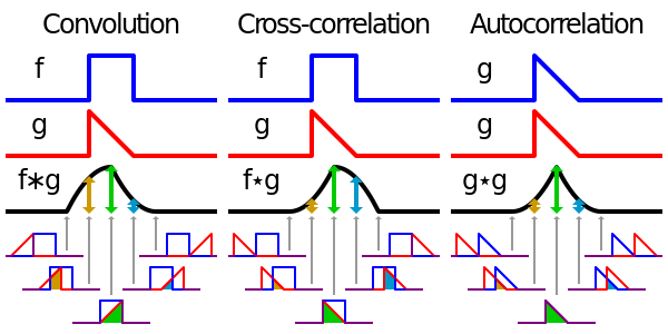
Convolution is the operation that ties the impulse response to the system's output for an arbitrary input. For an LTI system with impulse response $h(t)$ and input $x(t)$, the output is:

$y(t) = x(t) * h(t) = \int_{-\infty}^{\infty} x(\tau)\, h(t - \tau)\, d\tau$

Here's how to think through computing a convolution step by step:

1. Replace $t$ with a dummy variable $\tau$ in both signals, giving you $x(\tau)$ and $h(\tau)$.

2. Time-reverse the impulse response to get $h(-\tau)$.

3. Shift the reversed impulse response by $t$ to get $h(t - \tau)$.

4. Multiply $x(\tau)$ and $h(t - \tau)$ together for each value of $\tau$.

5. Integrate the product over all $\tau$. The result is $y(t)$ at that particular value of $t$.

6. Repeat for every value of $t$ you care about.

The reason this works is that any input can be thought of as a sum of scaled, shifted impulses. Linearity and time-invariance guarantee that the output is the corresponding sum of scaled, shifted impulse responses. Convolution is just the continuous version of that sum.

Step Response and Differential Equations

The step response and differential equations are closely related. You often find the step response by solving the system's differential equation with $x(t) = u(t)$ as the input.

The general form of a linear constant-coefficient ODE for an LTI system is:

$a_n\frac{d^n y(t)}{dt^n} + a_{n-1}\frac{d^{n-1} y(t)}{dt^{n-1}} + \cdots + a_1\frac{dy(t)}{dt} + a_0\, y(t) = b_m\frac{d^m x(t)}{dt^m} + b_{m-1}\frac{d^{m-1} x(t)}{dt^{m-1}} + \cdots + b_1\frac{dx(t)}{dt} + b_0\, x(t)$

The coefficients $a_i$ and $b_i$ are constants that define the system. The left side involves the output and its derivatives; the right side involves the input and its derivatives.

To solve one of these equations for a given input:

1. Find the homogeneous solution (set the right side to zero and solve the characteristic equation for its roots).
2. Find a particular solution that satisfies the full equation with the input present.
3. Combine them: the total solution is the sum of the homogeneous and particular solutions.
4. Apply initial conditions to determine any unknown constants.

For a first-order system like $\frac{dy(t)}{dt} + a_0\, y(t) = b_0\, x(t)$, the characteristic equation has one root, and the homogeneous solution is a single exponential. For a second-order system, you get two roots, which can be real and distinct, repeated, or complex conjugates. Each case produces different transient behavior (overdamped, critically damped, or underdamped, respectively).

The connection between all these tools is worth keeping in mind: the differential equation defines the system, the impulse response characterizes it, convolution uses that characterization to find outputs, and the step response gives you a practical snapshot of how the system performs.