13.1 Analog vs. digital signals

Analog and Digital Signals

Types of Signals

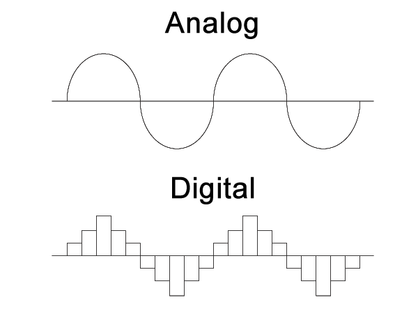
Analog signals represent information through continuous variations in amplitude or frequency over time. They can take on an infinite number of values within a range. Think of a temperature sensor outputting a voltage that smoothly rises and falls as the room warms and cools. Other common examples include sound waves, voltages from sensors, and traditional analog TV broadcasts.

Digital signals convey information using discrete levels at specific points in time. They're typically represented by binary digits (bits) with two possible states: 0 and 1. Because digital signals only need to distinguish between a small number of levels, they're much less susceptible to noise and distortion than analog signals. Examples include MP3 audio files, JPEG images, and digital television broadcasts.

A related distinction worth keeping straight:

• Continuous signals have values defined at every point in time. Analog signals are inherently continuous.
• Discrete signals have values defined only at specific time intervals. Digital signals are discrete, with a finite number of possible values at each sampling point.

Advantages and Disadvantages

Analog signals degrade more easily over distance and through noisy environments:

• Noise gets introduced by external sources (electromagnetic interference, for instance) or by the transmission medium itself.
• Distortion occurs from non-linear effects in the system, such as amplifier saturation.
• Attenuation is the gradual reduction in signal strength as it travels through a medium.

Digital signals have several practical advantages:

• They can be processed, stored, and transmitted more efficiently and reliably.
• Error detection and correction techniques help maintain signal integrity even over noisy channels.
• Encryption can secure digital data during transmission.

The tradeoff is that digital signals generally require more bandwidth to represent the same information. Higher sampling rates and more quantization levels are needed to faithfully capture the original analog signal. On top of that, the conversion processes themselves (analog-to-digital and digital-to-analog) introduce quantization errors and some latency.

Sampling and Quantization

Sampling Process

Sampling converts a continuous-time signal into a discrete-time signal by measuring its amplitude at regular intervals.

• The time between samples is the sampling period ($T_s$), and its reciprocal is the sampling frequency ($f_s$).
• The Nyquist-Shannon sampling theorem states that the sampling frequency must be at least twice the highest frequency component in the analog signal to avoid aliasing.
• Aliasing occurs when high-frequency components in the original signal get misinterpreted as lower-frequency components in the sampled version. This is an irreversible distortion if it happens during sampling.

Oversampling means using a sampling frequency much higher than the Nyquist rate. This has two practical benefits:

• It allows the use of simpler anti-aliasing filters with more gradual roll-off characteristics.
• After oversampling, decimation can reduce the sample rate back down while filtering out high-frequency noise picked up during conversion.

Quantization and Resolution

Quantization maps the continuous range of sampled amplitudes to a finite set of discrete values. Each discrete value is represented by a binary code.

The quantization step size ($\Delta$) is the smallest difference between two consecutive quantization levels:

$\Delta = \frac{V_{max} - V_{min}}{2^N}$

where $V_{max}$ and $V_{min}$ are the maximum and minimum values of the analog signal, and $N$ is the number of bits used for quantization.

Quantization introduces an irreversible error called quantization noise, which is the difference between the original analog value and its quantized representation. You can't get that lost information back.

The resolution of an ADC or DAC is the number of discrete values it can produce or measure:

• An $N$-bit converter has $2^N$ levels.
• Higher resolution means a smaller step size and lower quantization noise.
• For example, an 8-bit ADC with a 0–5V range has $2^8 = 256$ levels and a step size of $5V / 256 \approx 19.5 \text{ mV}$.

ADC and DAC

Analog-to-digital conversion (ADC) converts a continuous-time, continuous-amplitude signal into a discrete-time, discrete-amplitude signal. ADCs show up in digital audio recording, digital photography, data acquisition systems, and many other applications.

The ADC process works through three main stages:

1. Sample-and-hold circuit captures the instantaneous value of the analog signal at each sampling point and holds it constant long enough for the next stage to measure it.
2. Quantizer compares the held value to a set of reference voltages and determines which quantization level is closest.
3. Encoder converts the quantizer's output into a standard binary format (e.g., straight binary, two's complement, or Gray code).

Digital-to-analog conversion (DAC) is the reverse process, converting a discrete digital signal back into a continuous analog signal. DACs are used in audio playback, video display drivers, and control systems.

The DAC process also has three main stages:

1. Decoder converts the input binary code into control signals.
2. Binary-weighted current sources or resistors generate analog output levels proportional to the binary input.
3. Summing amplifier combines the individual outputs into a single continuous-time signal.

Signal Characteristics

Bandwidth

Bandwidth measures the range of frequencies present in a signal, or the range of frequencies a system can handle.

• For a low-pass signal, bandwidth is simply the highest frequency component present.
• For a bandpass signal, bandwidth is the difference between the highest and lowest frequency components.
• Bandwidth is measured in Hertz (Hz) or multiples like kHz, MHz, and GHz.

Bandwidth connects directly to sampling. The Nyquist-Shannon theorem tells you the minimum sampling rate for a bandlimited signal with maximum frequency $f_{max}$:

$f_s \geq 2f_{max}$

This minimum rate is called the Nyquist rate.

A system's bandwidth (whether it's an ADC, DAC, or communication channel) limits what frequencies it can accurately process. This is often specified by the -3 dB cutoff frequency, which is the frequency at which the output power drops to half the input power. For example, a 100 MHz oscilloscope can accurately measure signals with frequency components up to about 100 MHz.

Signal-to-Noise Ratio (SNR)

Signal-to-noise ratio (SNR) measures the relative strength of the desired signal compared to background noise. It's expressed in decibels (dB):

$SNR_{dB} = 10 \log_{10} \left(\frac{P_{signal}}{P_{noise}}\right)$

where $P_{signal}$ and $P_{noise}$ are the power of the signal and noise, respectively. A higher SNR means a cleaner signal; a lower SNR means more corruption from noise.

For digital systems, SNR is commonly used to evaluate ADC and DAC performance. An ideal $N$-bit ADC has a theoretical maximum SNR of:

$SNR_{max,dB} = 6.02N + 1.76$

This assumes quantization noise is uniformly distributed and uncorrelated with the input. In practice, actual SNR falls below this theoretical maximum because of thermal noise, clock jitter, and other non-ideal circuit behavior.

Several techniques can improve a system's SNR:

• Increase signal power by using a higher-gain amplifier or stronger transmitter.
• Reduce noise power through shielded cables, proper grounding, and low-noise components.
• Oversample and average multiple samples to reduce the effect of random noise.
• Apply error correction codes and digital signal processing techniques to mitigate noise impact.