17.3 Convolution and correlation

Convolution

Convolution Integral and Sum

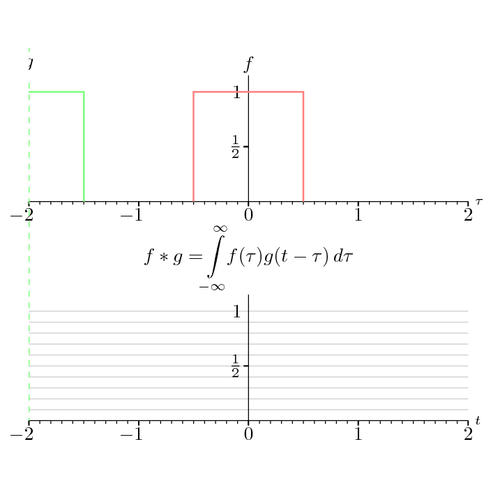
Convolution is how you find the output of a linear time-invariant (LTI) system when you know two things: the input signal and the system's impulse response. The impulse response is simply what the system outputs when you feed it the shortest possible "spike" input.

For continuous-time systems, the convolution integral is:

$y(t) = \int_{-\infty}^{\infty} x(\tau) \, h(t - \tau) \, d\tau$

where $x(t)$ is the input signal and $h(t)$ is the impulse response. That "spike" input is modeled as the Dirac delta function $\delta(t)$, an idealized pulse with infinite height, zero width, and an area of 1.

For discrete-time systems, the convolution sum does the same job:

$y[n] = \sum_{k=-\infty}^{\infty} x[k] \, h[n - k]$

Here the "spike" input is the Kronecker delta $\delta[n]$, which equals 1 at $n = 0$ and 0 everywhere else.

In both cases, the idea is the same: you're building the output sample-by-sample (or point-by-point) by sliding the flipped impulse response across the input and summing up the overlapping products.

System Response and Impulse Response

If you know a system's impulse response $h(t)$ (or $h[n]$), you know everything about how that LTI system behaves. Any input you throw at it can be broken into a collection of scaled, shifted impulses, and the output is the sum of the corresponding scaled, shifted impulse responses. That's exactly what the convolution operation computes.

This is why impulse responses matter so much in practice. Filters, equalizers, and control systems are all characterized by their impulse responses. Measure or design $h$, and you can predict the output for any input.

Steps to compute convolution (graphical method):

1. Write out $x(\tau)$ and $h(\tau)$.

2. Flip $h(\tau)$ to get $h(-\tau)$.

3. Shift the flipped version by $t$ to get $h(t - \tau)$.

4. Multiply $x(\tau)$ and $h(t - \tau)$ together.

5. Integrate (or sum, for discrete-time) the product over all $\tau$.

6. Repeat for each value of $t$ you need.

Correlation

Cross-Correlation and Auto-Correlation

While convolution asks "what does this system output?", correlation asks "how similar are these two signals?"

Cross-correlation measures the similarity between two signals as you slide one past the other in time. The continuous-time cross-correlation of $x(t)$ and $y(t)$ is:

$R_{xy}(\tau) = \int_{-\infty}^{\infty} x(t) \, y(t + \tau) \, dt$

The variable $\tau$ is the lag, the time-shift applied to one signal. Where $R_{xy}(\tau)$ peaks tells you the lag at which the two signals line up best. This is exactly how radar and sonar systems estimate the distance to a target: they transmit a pulse, receive the echo, and cross-correlate to find the time delay.

Auto-correlation is the cross-correlation of a signal with itself:

$R_{xx}(\tau) = \int_{-\infty}^{\infty} x(t) \, x(t + \tau) \, dt$

Auto-correlation always peaks at $\tau = 0$ (a signal is most similar to itself with no shift). Its real usefulness is in revealing repeating patterns. If a signal has a periodic component, the auto-correlation will show peaks at lags equal to the period. Applications include pitch detection in audio and identifying cyclic behavior in data.

Properties of Correlation

A few properties make correlation easier to work with:

• Time-shifting: If you shift one of the input signals by some amount $t_0$, the cross-correlation function shifts by the same amount. The shape doesn't change, only where the peak lands.
• Symmetry: Cross-correlation is not symmetric in general: $R_{xy}(\tau) = R_{yx}(-\tau)$. Swapping which signal you shift is the same as flipping the lag axis. Auto-correlation, however, is symmetric: $R_{xx}(\tau) = R_{xx}(-\tau)$.
• Duality with convolution: Cross-correlation of $x$ and $y$ equals the convolution of $x$ with the time-reversed version of $y$. This means you can compute correlation using the same fast algorithms built for convolution, including the Fast Fourier Transform (FFT). In the frequency domain, cross-correlation becomes $R_{xy}(f) = X(f) \cdot Y^*(f)$, where $Y^*(f)$ is the complex conjugate of $Y(f)$.