5.3 Job Shop Scheduling and Sequencing

Job Shop Production Environments

Characteristics and Layout

Job shop production handles custom products in small batches, where each product follows its own unique route through different workstations. This makes it fundamentally different from assembly lines or flow shops, where every product takes the same path.

• High product variety, low volume defines the job shop. You might produce dozens of different part types, but only a handful of each.
• Equipment is flexible and workers are skilled across multiple tasks, which is what makes all that variety possible.
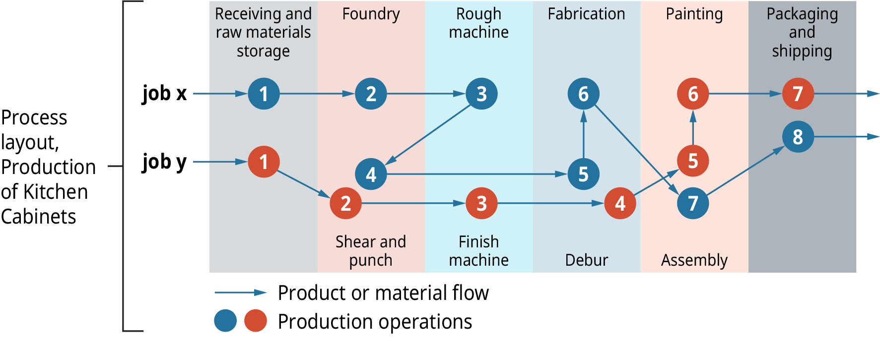
• The physical layout is functional (also called a process layout), meaning similar machines are grouped together: all milling machines in one area, all lathes in another, welding stations in a third. Jobs travel between these groups based on their specific routing.
• Because every job can take a different path through the shop, material handling and routing get complicated fast.

Challenges and Complexities

The flexibility that makes job shops useful also makes them hard to manage:

• Process flows vary from job to job, and processing times differ, so there's no single "standard" schedule to follow.
• Frequent machine setups are needed because you're constantly switching between different product specifications.
• Multiple objectives compete with each other. Minimizing makespan, meeting due dates, and keeping machines busy don't always point to the same schedule.
• Work-in-process (WIP) inventory tends to pile up, and lead times run longer than in more streamlined production systems.
• Bottlenecks shift around depending on the current job mix, making capacity planning unpredictable.
• Schedules need frequent adjustment as new jobs arrive, priorities change, or disruptions occur.

Job Shop Scheduling Techniques

Priority Rules and Dispatching

Priority rules are simple decision rules that determine which job gets processed next at a workstation. They're easy to implement and widely used in practice, even though they don't guarantee an optimal schedule.

Common priority rules include:

• Shortest Processing Time (SPT): Process the job with the shortest operation time first. This tends to minimize average flow time and reduce the number of jobs waiting in the system.
• Earliest Due Date (EDD): Prioritize the job whose due date is closest. This is effective for minimizing maximum tardiness (how late the worst-case job is).
• First-Come-First-Served (FCFS): Process jobs in the order they arrive. Simple and perceived as "fair," but generally performs poorly on efficiency metrics.
• Longest Processing Time (LPT): Process the longest job first. This can be useful when you want to minimize makespan on parallel machines, since it avoids leaving a long job stranded at the end.
• Critical Ratio (CR): Calculated as $CR = \frac{\text{Time Until Due Date}}{\text{Remaining Processing Time}}$. A ratio below 1.0 means the job is behind schedule and needs priority. Jobs with the lowest CR get scheduled first. This rule dynamically balances urgency against remaining workload.

Dispatching is the real-time act of assigning jobs to machines based on current shop status, available capacity, and whichever priority rule you're using. Gantt charts are the standard visual tool for representing these schedules, showing which job is on which machine over time. They make it easy to spot conflicts, idle periods, and bottlenecks at a glance.

Advanced Scheduling Methods

When priority rules aren't enough, more sophisticated methods come into play:

• Shifting Bottleneck Procedure: Schedules one machine at a time, always tackling the current bottleneck machine next. After each machine is scheduled, it re-evaluates which machine is now the bottleneck. This iterative approach produces strong results for moderately sized problems.
• Simulation-based scheduling: Builds a computer model of the job shop and runs different scheduling scenarios to compare performance before committing to one. Particularly useful for capturing the dynamic, stochastic nature of real shops.
• Genetic Algorithms (GAs): Maintain a "population" of candidate schedules and improve them over many iterations using operators inspired by evolution (selection, crossover, mutation).
• Tabu Search: A local search method that keeps a memory of recently visited solutions (the "tabu list") to avoid cycling back and getting stuck in local optima.
• Constraint Programming: Defines the scheduling problem as a set of constraints (machine capacity, job precedence, time windows) and uses specialized solvers to find feasible or optimal solutions efficiently.

Job Shop Scheduling Performance

Evaluation Metrics

You need clear metrics to judge whether a schedule is good. The most common ones:

• Makespan ($C_{max}$): Total time from when the first job starts to when the last job finishes. Lower is better since it means all work gets done sooner.
• Total flow time: The sum of completion times across all jobs. Minimizing this reduces the average time a job spends in the system. Average flow time is just total flow time divided by the number of jobs.
• Tardiness: How late jobs are relative to their due dates. A job finished on or before its due date has zero tardiness (tardiness is never negative, unlike lateness, which can be). You might track average tardiness, maximum tardiness, or the number of tardy jobs.
• Machine utilization: The percentage of time machines are actively processing, as opposed to sitting idle or being set up. Higher utilization generally means better resource use.
• Work-in-process (WIP) levels: The count of partially completed jobs in the system at any point. High WIP ties up capital and floor space.

These metrics can be evaluated deterministically (assuming everything goes exactly as planned) or stochastically (accounting for variability in processing times, machine breakdowns, etc.). Real shops almost always need stochastic analysis.

Performance Analysis Techniques

• Sensitivity analysis tests how much your schedule's performance changes when input parameters shift (e.g., what happens if processing times are 10% longer than estimated?).
• Benchmarking compares your scheduling method's results against known optimal solutions (for small problems) or published industry standards.
• Robustness analysis measures how well a schedule holds up when disruptions occur, such as machine breakdowns or rush orders.
• Trade-off analysis explicitly examines the tension between conflicting objectives. For example, minimizing makespan might require more setups, which increases costs.
• Simulation studies run scheduling methods over extended time horizons with realistic variability to assess long-term, steady-state performance.
• Statistical methods like ANOVA or regression analysis can quantify which factors (priority rule choice, job mix, machine count) most significantly affect scheduling outcomes.

Job Sequencing Optimization

Exact Methods for Optimal Sequencing

Exact methods guarantee an optimal solution, but they come with computational limits. Job shop scheduling is NP-hard for most nontrivial cases, which means computation time can grow explosively as problem size increases.

• Johnson's Algorithm finds the optimal job sequence for a two-machine flow shop problem (every job visits Machine 1 then Machine 2), minimizing makespan. The steps are:

  1. List the processing time for each job on both machines.
  2. Find the smallest processing time across all jobs and machines.
  3. If that time is on Machine 1, place the job as early as possible in the sequence. If it's on Machine 2, place it as late as possible.
  4. Remove that job from the list and repeat until all jobs are sequenced.
  5. If there's a tie (equal processing times on both machines), either position works.

  Johnson's Algorithm can be extended to certain restricted three-machine cases (where the middle machine is never the bottleneck), but it doesn't generalize to arbitrary job shops.

• Branch and Bound systematically explores the space of possible sequences, using lower bounds to prune branches that can't beat the best solution found so far. Practical for small to medium problems, but computation time grows rapidly with problem size.

• Integer Programming (IP) formulates the scheduling problem as a mathematical optimization model with binary decision variables (e.g., $x_{ij} = 1$ if job $i$ precedes job $j$ on a machine). Commercial solvers like CPLEX or Gurobi can handle these, though large instances may be intractable.

• Critical Path Method (CPM) identifies the longest chain of dependent operations, which determines the minimum possible makespan. Any delay on the critical path delays the entire schedule.

• Disjunctive graph models represent job shop problems as graphs where nodes are operations and edges represent precedence and machine-sharing constraints. Solving the problem means resolving the "disjunctive" (either/or) arcs on shared machines to find the sequence that minimizes makespan.

Heuristic and Approximation Techniques

For larger or more complex problems, heuristics find good (though not guaranteed optimal) solutions in reasonable time.

• Shifting Bottleneck Procedure is one of the best-known heuristics for job shop sequencing, producing near-optimal results on many benchmark problems.
• Genetic Algorithms evolve a population of candidate sequences through selection, crossover, and mutation. They explore broadly and handle large solution spaces well.
• Dominant sequences are job orderings that can be proven optimal or near-optimal under specific conditions. For example, SPT is provably optimal for minimizing total flow time on a single machine, so in that setting you don't need a more complex method.
• Local search methods like Simulated Annealing and Tabu Search start with an initial sequence and iteratively swap or rearrange jobs, accepting improvements and occasionally accepting worse moves to escape local optima.
• Constructive heuristics build a schedule from scratch, adding one job at a time using a priority rule or greedy criterion.
• Rolling horizon approaches optimize the schedule over a short time window, then shift the window forward and re-optimize as new jobs and updated information arrive. This is how many real shops operate in practice, since the full problem is too large and too uncertain to solve all at once.