System performance evaluation through simulation
Simulation output analysis is how you figure out what your simulation results actually mean. Running a simulation once and reading off a number isn't enough. Because simulations use random inputs, your outputs are random too, and you need statistical tools to separate real patterns from noise. This topic covers how to design simulation experiments, analyze the output data, determine how many runs you need, and use optimization to find the best system configuration.
Experimental design for simulation studies
Before running a simulation, you need a plan for which inputs to vary and how to vary them. That plan is your experimental design, and it directly affects whether you can draw valid conclusions from your results.
Factorial designs let you evaluate multiple factors and their interactions at the same time. For example, if you're simulating a manufacturing line, you might vary both the number of machines (2 vs. 4) and the buffer size (5 vs. 10). A full factorial design tests every combination, so you can see not just the effect of each factor alone, but whether they interact (maybe adding machines only helps when buffers are large enough).
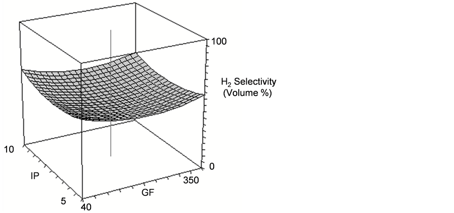
Response surface methodology (RSM) goes a step further. Instead of testing just a few levels of each factor, RSM fits a mathematical surface to your results, helping you map out how outputs change across a range of inputs. This is especially useful when you're trying to find an optimal operating point.
Variance reduction techniques make your simulation experiments more efficient by reducing the randomness in your output without adding more runs:
- Common random numbers: Use the same random number streams across different configurations so that differences in output reflect actual system differences, not just random variation.
- Antithetic variates: Pair each run with a "mirror" run that uses complementary random numbers, which tends to reduce the variance of the average.
Three core principles keep your experiments valid:
- Randomization prevents systematic bias in how you assign experimental conditions
- Replication gives you multiple observations so you can estimate variability
- Blocking groups similar experimental conditions together to control for known sources of variation
Sensitivity analysis and scenario analysis round out the design toolkit. Sensitivity analysis tells you which input parameters have the biggest impact on your output, helping you focus your attention on what matters most. Scenario analysis evaluates specific "what-if" situations (e.g., what if demand doubles next quarter?) to see how the system behaves under different conditions.
Advanced simulation analysis techniques
Once you have output data, several techniques help you interpret it correctly.
Steady-state analysis applies when you're simulating a system that runs continuously (like a call center). The simulation needs time to "warm up" before its output represents normal operating conditions. You need to identify and remove this initial transient period so it doesn't bias your results. Welch's method (covered below) is a common way to estimate how long the warm-up lasts.
Autocorrelation is a challenge unique to simulation. Within a single long run, consecutive observations are often correlated (a busy period tends to be followed by another busy period). You can check for this using autocorrelation function (ACF) plots. If observations are correlated, standard statistical formulas that assume independence will underestimate your uncertainty.
Multivariate analysis handles situations where you're tracking multiple performance measures at once (e.g., throughput, average wait time, and utilization). These measures are often correlated, so analyzing them separately can be misleading.
Hypothesis testing lets you make formal comparisons. For instance, you might test whether a proposed layout change actually reduces average cycle time compared to the current layout, or you might validate your simulation by comparing its output to real-world data.
Data analysis for simulation outputs
Statistical methods for output analysis
The goal of output analysis is to take the raw numbers from your simulation runs and turn them into reliable estimates with known precision.
Confidence intervals are the primary tool. Rather than reporting a single number (e.g., "average wait time = 4.2 minutes"), you report a range that accounts for uncertainty (e.g., "average wait time = 4.2 ± 0.3 minutes at 95% confidence"). This tells decision-makers how much to trust the estimate.
For terminating simulations (ones with a natural start and end, like simulating one 8-hour shift), you run multiple independent replications and compute the confidence interval from the sample of replication averages.
For steady-state simulations (ones meant to represent long-run behavior), you often use a single long run. The batch means method divides that long run into consecutive batches, treats each batch average as an approximately independent observation, and uses those batch averages to estimate variance and build confidence intervals.
Determining how many replications you need is a practical concern. Two common approaches:
- Coefficient of variation method: Use a small pilot study to estimate variability, then calculate roughly how many replications you'll need to hit your target precision.
- Sequential sampling: Start running replications and check your confidence interval width after each one. Stop when you've reached your desired relative precision (e.g., the half-width of the confidence interval is within 5% of the estimated mean).
Statistical foundations
Two theorems from probability justify why these methods work:
- The Law of Large Numbers guarantees that your sample average converges to the true mean as you increase the number of replications.
- The Central Limit Theorem tells you that the distribution of the sample average becomes approximately normal regardless of the underlying distribution, which is why confidence interval formulas based on the normal (or t) distribution are valid.
Welch's method helps estimate the warm-up period for steady-state simulations. You run several replications, average the output across replications at each time point, and apply a moving average to smooth the result. The point where the smoothed curve levels off suggests where the transient period ends and steady-state begins.
Optimal Computing Budget Allocation (OCBA) is a more advanced technique for when you're comparing multiple system configurations. Instead of giving every configuration the same number of runs, OCBA allocates more runs to configurations that are harder to distinguish (close in performance or high in variance). This makes better use of your computing budget.
Simulation-based optimization
Optimization techniques in simulation
Sometimes you don't just want to evaluate a system; you want to find the best configuration. Simulation-based optimization combines simulation with search algorithms to do exactly that.
The challenge is that you can't write a neat closed-form equation for your objective function. The simulation is the function, and each evaluation requires running the model (which takes time and produces noisy results).
Metaheuristic algorithms search through large, complex solution spaces where exhaustive search isn't feasible:
- Genetic algorithms maintain a "population" of candidate solutions that evolve over generations through selection, crossover, and mutation. They're good at exploring diverse regions of the solution space.
- Simulated annealing starts with a high "temperature" that allows accepting worse solutions (to escape local optima), then gradually cools down to converge on a good solution.
Response surface methodology (RSM) can also serve an optimization role. By fitting a mathematical model to simulation results, you can use calculus or numerical methods on the fitted surface to find the optimum, which is much cheaper than running more simulations.
Ranking and selection procedures apply when you have a finite set of candidate designs (e.g., 10 possible layouts). These statistical procedures determine how many simulation runs each design needs so you can confidently identify the best one, controlling the probability of making a wrong selection.
Sample path optimization (also called stochastic approximation) works for problems with continuous decision variables. It fixes the random number streams and optimizes over a single "sample path," then repeats with different streams to account for randomness.
Constraint handling and multi-objective optimization
Real-world problems almost always involve constraints (budget limits, space restrictions, minimum service levels). Constraint handling techniques ensure that the optimization search only considers feasible solutions, or penalizes infeasible ones to steer the search back toward valid configurations.
Many real problems also have conflicting objectives. For example, you might want to minimize cost and maximize throughput, but these goals pull in opposite directions. Multi-objective optimization doesn't produce a single "best" answer. Instead, it generates a set of Pareto-optimal solutions, where no objective can be improved without worsening another. Decision-makers then choose from this set based on their priorities.