Linear Programming in Standard Form
Before the Simplex Method can solve a linear programming (LP) problem, that problem needs to be in standard form. Standard form has three requirements: the objective function is a maximization, all constraints are equalities, and all variables are non-negative.
Converting Constraints and the Objective Function
Here's how to convert any LP problem into standard form:
- Inequality constraints (≤): Add a slack variable to turn the inequality into an equality. Slack variables represent unused resources and are always non-negative.
- Inequality constraints (≥): Subtract a surplus variable and add an artificial variable. The surplus captures how much you exceed the minimum, while the artificial variable is a mathematical trick to get a starting feasible solution (it gets driven to zero during solving).
- Minimization objectives: Multiply the entire objective function by to convert it into a maximization problem.
- Unrestricted variables: If a variable can be negative, replace it with , where both and .
The constraint coefficient matrix should have full row rank, meaning no constraint is a redundant combination of others.
Example of Standard Form Conversion
- Original constraint:
- Standard form: , where is a slack variable
- Original objective: Minimize
- Standard form: Maximize
- Unrestricted variable: has no sign restriction
- Standard form: , with
Simplex Algorithm for Optimization
The Simplex Method solves LP problems by moving along the edges of the feasible region from one corner point (basic feasible solution) to an adjacent one, improving the objective function at each step. It's efficient because it doesn't check every corner point; it strategically picks the most promising direction.
Iterative Process and Basic Concepts
The algorithm follows these steps:
- Find an initial basic feasible solution. Set all non-basic variables to zero and solve for the basic variables. Slack variables often serve as the initial basis.
- Check for optimality. Look at the reduced costs (the coefficients in the objective function row of the tableau). For a maximization problem, if all reduced costs are non-negative (no negative entries), you've found the optimal solution. Stop here.
- Select the entering variable. Choose the non-basic variable with the most negative reduced cost. This variable will enter the basis because increasing it improves the objective value the most.
- Select the leaving variable (minimum ratio test). For each positive entry in the entering variable's column, divide the right-hand side value by that entry. The row with the smallest ratio identifies the leaving variable. This test ensures the solution stays feasible.
- Pivot. Use row operations to update the tableau so the entering variable replaces the leaving variable in the basis.
- Repeat from Step 2.
A few things to watch for:
- Degeneracy occurs when a basic variable equals zero. This can cause the algorithm to cycle through the same solutions without improving. Special rules (like Bland's rule) prevent this.
- Unboundedness is detected when no positive entries exist in the entering variable's column during the ratio test, meaning the objective can increase without limit.
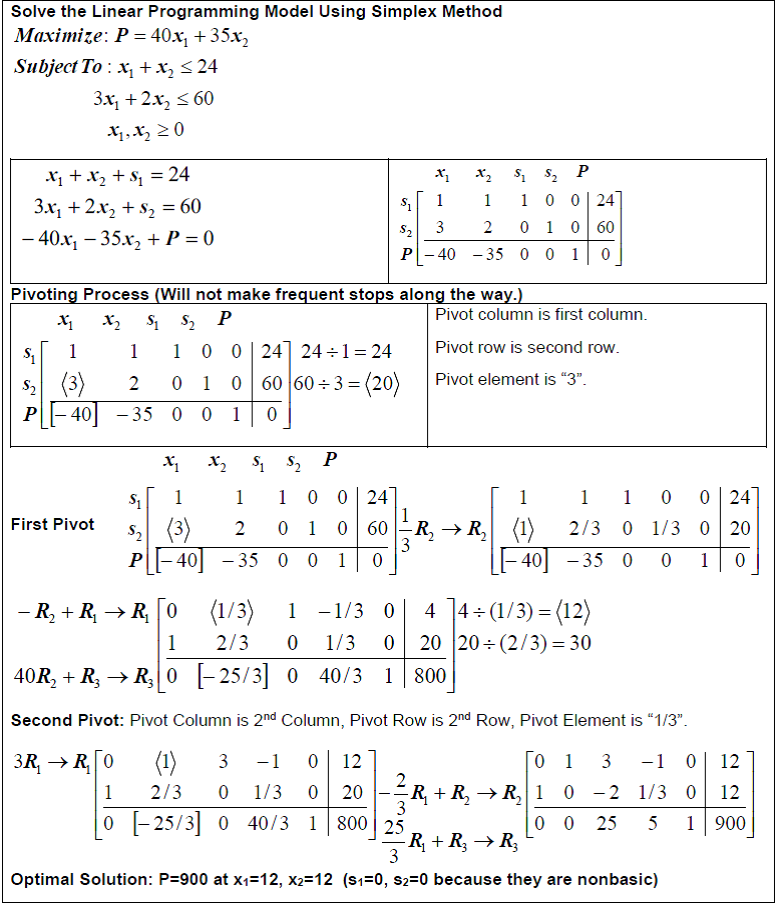
Simplex Tableau and Pivot Operations
The simplex tableau organizes all the information you need: objective function coefficients across the top row, constraint coefficients in the body, and right-hand side (RHS) values in the last column.
To perform a pivot:
- Identify the pivot element at the intersection of the entering variable's column and the leaving variable's row.
- Divide the entire pivot row by the pivot element so the pivot element becomes 1.
- Use row operations to make all other entries in the pivot column equal to zero:
Quick example: Suppose the pivot element is 2.
- Pivot row: → after dividing by 2:
- Old row: → new row:
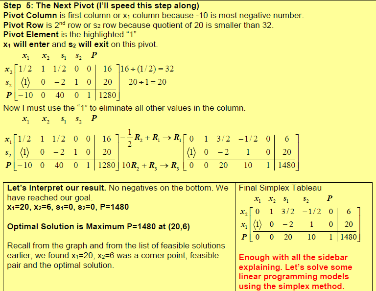
Continue pivoting until all reduced costs in the objective row are non-negative.
Optimal Solutions and Shadow Prices
Interpreting the Final Simplex Tableau
Once the algorithm terminates, the final tableau tells you everything about the solution:
- Optimal variable values: Basic variables' values appear in the RHS column. Non-basic variables equal zero.
- Optimal objective value: Found in the bottom-right cell of the tableau.
- Reduced costs: The entries in the objective row for non-basic variables. A reduced cost tells you how much the objective value would decrease per unit if you forced that variable into the solution.
- Slack/surplus variable values: If a slack variable is zero, its corresponding constraint is binding (the resource is fully used). If it's positive, there's leftover capacity.
Economic Interpretation of Shadow Prices
Shadow prices (also called dual variables or dual prices) appear in the objective row of the final tableau, in the columns corresponding to the original slack/surplus variables. They answer a practical question: how much is one more unit of a resource worth?
- A positive shadow price means the objective value would improve if that constraint were relaxed (more of that resource were available).
- A zero shadow price means the constraint is non-binding, so adding more of that resource wouldn't help right now.
For example, if the shadow price for a raw material constraint is , then each additional unit of that raw material would increase the optimal objective value by (within the range of feasibility).
Sensitivity Analysis of Parameters
Real-world data is rarely exact. Sensitivity analysis tells you how much the problem's parameters can change before the current optimal solution or basis breaks down, without having to re-solve the entire problem from scratch.
Ranges of Optimality and Feasibility
Two key ranges define the stability of your solution:
- Range of optimality: How much an objective function coefficient can change while the current set of basic variables (the current solution) remains optimal. The variable values may change, but the same variables stay in the basis.
- Range of feasibility: How much a right-hand side (RHS) value can change while the current basis remains feasible. Within this range, the shadow prices remain valid.
For simultaneous changes to multiple RHS values, use the 100% rule: calculate each change as a percentage of its allowable increase or decrease, then sum the percentages. If the total is under 100%, the current basis is guaranteed to remain feasible.
If changes fall outside these ranges, you'll need to re-solve the problem (or use the dual simplex method to recover).
Examples of Sensitivity Analysis
- Objective coefficient range: The coefficient of can vary from 2 to 5 without changing which variables are in the optimal basis.
- RHS range: Resource 1 can increase by 10 units or decrease by 5 units while the current basis (and shadow prices) remain valid.
- Simultaneous changes using the 100% rule: Suppose Resource 1's allowable increase is 10 and Resource 2's allowable increase is 5. If you increase Resource 1 by 3 and Resource 2 by 2, the percentages are , or 70%. Since 70% < 100%, the optimal basis is unchanged.
Duality in Linear Programming
Every LP problem (the primal) has a companion problem called the dual. The dual isn't just a mathematical curiosity; it provides an economic interpretation of the primal and connects directly to shadow prices.
Primal-Dual Relationships
The core theorems that link primal and dual:
- Weak duality: Any feasible solution to the dual gives a bound on the primal's optimal value (an upper bound for maximization, a lower bound for minimization). This is useful for checking whether a solution is close to optimal.
- Strong duality: If either the primal or dual has an optimal solution, both do, and their optimal objective values are equal.
- Complementary slackness: At optimality, if a primal constraint has slack (is non-binding), the corresponding dual variable is zero, and vice versa. This links shadow prices directly to binding constraints.
The dual simplex method works with the primal tableau but effectively solves the dual. It's especially useful for re-optimization after sensitivity analysis changes make the current solution infeasible.
Constructing and Interpreting Dual Problems
To build the dual from the primal, follow these conversion rules:
| Primal (Maximize) | Dual (Minimize) |
|---|---|
| Objective coefficients | RHS values |
| RHS values | Objective coefficients |
| constraints | dual variables |
| Variables | constraints |
| Inequality direction | Reverses |
Example:
- Primal: Maximize subject to , , with
- Dual: Minimize subject to , , with
The dual variables and correspond to the two primal constraints. At optimality, their values equal the shadow prices from the primal's final tableau.