10.1 Discrete-Event Simulation Concepts

Discrete-event simulation fundamentals

Discrete-event simulation (DES) lets you model systems where changes happen at specific moments rather than continuously. Think of a factory floor: nothing changes between events, but when a part arrives at a machine or a worker finishes an assembly, the whole system state updates at once. This makes DES especially useful for analyzing processes in manufacturing, healthcare, logistics, and service operations.

By breaking a system into its core components, you can build a model, run it many times, and use the results to make better decisions about staffing, layout, scheduling, and more.

Key components and concepts

A DES model is built from a handful of building blocks. Understanding each one is essential before you try to build or interpret a simulation.

• Entities are the objects flowing through the system (customers in a bank, parts on an assembly line). Each entity can carry attributes that define its characteristics, like a customer's arrival time or a part's priority level.
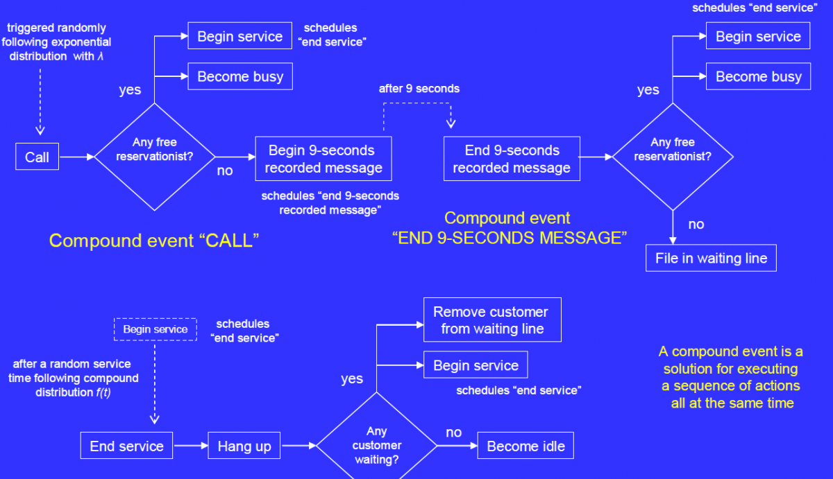
• Events are instantaneous occurrences that change the system state. Common examples: an entity arriving, a machine finishing a job, or a server becoming free.
• Resources provide service to entities. A resource can be a machine, a nurse, a forklift. At any moment, a resource is in a state like idle, busy, or down (broken/under maintenance).
• Queues hold entities that are waiting for a resource to become available or for some condition to be met. Queue behavior (first-in-first-out, priority-based, etc.) can significantly affect performance.
• Simulation clock tracks time in the model. Unlike a wall clock, it doesn't tick in fixed increments. Instead, it jumps forward from one event to the next, skipping over idle periods entirely.
• Random number generation and statistical distributions introduce the variability you see in real systems. Service times might follow an exponential distribution; arrival patterns might follow a Poisson process. Without this randomness, the model wouldn't capture real-world uncertainty.

Simulation mechanics and time management

The engine that drives a DES model is the event list (sometimes called the future event list). Here's how the core simulation loop works:

1. The simulation starts with an initial event on the event list (e.g., "first customer arrives at time 0").
2. The clock advances to the time of the next event on the list.
3. That event executes, updating the system state (e.g., a customer enters a queue, a machine starts processing).
4. The event may schedule new future events (e.g., "machine finishes processing at time 4.7").
5. Steps 2–4 repeat until a termination condition is met.

Termination conditions can be reaching a set clock time (e.g., simulate 8 hours), processing a target number of entities, or the system reaching a particular state.

A few additional mechanics to know:

• Conditional events don't have a pre-set time. They trigger when the system reaches a certain condition, like "start serving the next customer when the server becomes idle."
• Simultaneous events (two events scheduled for the exact same time) are resolved using priority rules or tie-breaking logic defined by the modeler.
• Because the state only updates at event times, DES is computationally efficient. The simulation skips all the "nothing happening" time between events.

Applications of discrete-event simulation

Manufacturing and supply chain

• Production systems: DES helps optimize scheduling and resource allocation on assembly lines and in job shops. You can test different sequencing rules (shortest job first, earliest due date) without disrupting real production.
• Supply chain management: Models can evaluate inventory policies (how much to order, when to reorder), compare distribution network designs, and identify bottlenecks in logistics operations.
• Warehouse operations: Simulating order-picking strategies, facility layouts, and material handling systems helps find configurations that reduce travel time and increase throughput.

Service industries and transportation

• Healthcare: Hospitals use DES to model patient flow through emergency departments, clinics, and surgical suites. The goal is often to reduce wait times and plan staffing or bed capacity.
• Transportation: Traffic flow at intersections, airport terminal operations (check-in, security, boarding), and public transit scheduling are all common DES applications.
• Customer service: Call centers simulate different staffing levels and routing rules to balance service quality against labor costs.

Project management and complex systems

• Project management: DES can model task durations with uncertainty, analyze critical paths under variable conditions, and assess the risk of schedule overruns.
• Financial systems: Models simulate market behavior and trading strategies to evaluate risk.
• Environmental systems: Simulations of pollution dispersion or ecological processes help predict outcomes under different policy scenarios.

Building discrete-event simulation models

Modeling approaches

There are several ways to structure the logic of a DES model. Each has trade-offs in terms of intuitiveness and flexibility.

• Event scheduling approach: You explicitly define each event type and write the logic for what happens when each event occurs. This gives you fine-grained control but requires more programming effort.
• Process interaction approach: You describe the system from the entity's perspective, modeling its flow through a sequence of steps (arrive, seize resource, delay, release resource). Most commercial simulation software (Arena, Simio, FlexSim) uses this approach because it maps naturally to flowcharts.
• Activity scanning approach: The model checks, at each time advance, which activities have their start conditions met. This works well for systems with complex, state-dependent behaviors but can be less computationally efficient.
• Three-phase approach: Combines event scheduling with activity scanning. Phase 1 advances the clock, Phase 2 executes scheduled events, and Phase 3 scans for conditional activities. This balances efficiency and flexibility.

For an intro course, the process interaction approach is the one you'll most likely use in software labs.

Model development process

Building a credible simulation model follows a structured process:

1. Define the scope: Set system boundaries and identify the key performance metrics you want to measure (throughput, average wait time, utilization, etc.).
2. Choose the level of detail: Decide what to model explicitly and what to simplify. Not every real-world detail needs to be in the model.
3. Collect and analyze input data: Gather real data on arrival rates, service times, breakdown frequencies, etc. Fit statistical distributions to this data.
4. Build the model: Implement the logic using your chosen modeling approach and software tool.
5. Verify: Check that the model runs as you intended. This is debugging: does the code do what you think it does?
6. Validate: Check that the model accurately represents the real system. Compare outputs to historical data or get expert review. Verification asks "did we build the model right?" while validation asks "did we build the right model?"
7. Document: Record all assumptions, limitations, data sources, and implementation choices. Future you (and your team) will thank you.

Analyzing discrete-event simulation models

Because DES models involve randomness, you can't draw conclusions from a single run. You need multiple replications (independent runs with different random number seeds) and proper statistical analysis.

Output analysis techniques

• Confidence intervals: Running multiple replications lets you calculate confidence intervals for your performance metrics. A single average from one run tells you very little; a 95% confidence interval from 30 runs tells you a lot more.
• Hypothesis testing: Use statistical tests to compare two system configurations (e.g., "does adding a second server significantly reduce average wait time?").
• Steady-state analysis: If you're modeling a system that runs continuously (like a 24/7 call center), you need to account for initialization bias. The early portion of the simulation, before the system "warms up" to typical operating conditions, should be discarded from your analysis.
• Variance reduction techniques: Methods like common random numbers (using the same random number streams across scenarios so differences are due to the design change, not randomness) and antithetic variates help you get more precise estimates without needing as many replications.

Performance evaluation and optimization

Common metrics to track in a DES model:

• Throughput: how many entities complete the process per unit time
• Cycle time: how long an entity spends in the system from entry to exit
• Resource utilization: the fraction of time a resource is busy
• Queue length and waiting time: how many entities are waiting and for how long

With these metrics in hand, you can:

• Run sensitivity analysis to see which input parameters have the biggest impact on outputs. If doubling the arrival rate barely changes wait times but a 10% increase in service time causes a spike, that tells you where to focus improvement efforts.
• Conduct scenario analysis by comparing results across different configurations (e.g., 2 servers vs. 3 servers, different queue disciplines).
• Use visualization tools like animated simulations and statistical charts to communicate findings and spot unexpected behaviors.
• Apply optimization techniques (response surface methodology, genetic algorithms) to search for the best system configuration when you have many decision variables.

Advanced analysis methods

These go a step beyond standard output analysis and are worth being aware of at the intro level:

• Metamodeling: Creating a simplified mathematical approximation (like a regression equation) of the simulation's input-output relationship. This lets you explore the design space quickly without running the full simulation every time.
• Design of experiments (DOE): A structured way to vary multiple input factors simultaneously so you can understand their individual and combined effects efficiently, rather than changing one factor at a time.
• Rare event simulation: Special techniques for estimating the probability of low-frequency, high-impact events (e.g., a system failure that happens once in 10,000 hours) without needing impossibly long simulation runs.
• Machine learning integration: Using ML algorithms to detect patterns in large volumes of simulation output or to build predictive models from simulation data.