2.2 Linear Programming Formulation and Graphical Solution

Formulating Linear Programs

Key Components of Linear Programming

Linear programming (LP) finds the best possible outcome from a mathematical model with linear relationships. You're trying to maximize or minimize some quantity while working within real-world limits.

Every LP problem has the same building blocks:

• Decision variables represent the quantities you're trying to determine. These are what you solve for (e.g., $x_1$, $x_2$, $x_3$).
• Objective function expresses your goal as a linear equation using the decision variables. This is what you want to maximize (like profit) or minimize (like cost).
• Constraints are linear inequalities or equations that represent limitations, such as resource availability, production capacity, or demand requirements.
• Non-negativity constraints require that decision variables be zero or positive ($x_1 \geq 0$, $x_2 \geq 0$), since negative quantities of products or shipments don't make sense.
• Slack variables get added to "less than or equal to" constraints to convert them into equalities (e.g., $2x_1 + 3x_2 \leq 100$ becomes $2x_1 + 3x_2 + s_1 = 100$). Surplus variables do the same for "greater than or equal to" constraints by subtracting from the left side.

Process of Formulating LP Problems

Translating a word problem into a mathematical LP model follows a consistent process:

1. Identify the decision variables. Ask yourself: what quantities does the decision-maker control?
2. Define the objective function. Write a linear expression that captures the goal (profit, cost, time, etc.) in terms of those variables.
3. Express each constraint as a linear inequality or equation. Every resource limit, capacity restriction, or requirement becomes one constraint.
4. Add non-negativity constraints for all decision variables.
5. Review the formulation. Check that units are consistent, no constraints are missing, and the model matches the original problem.

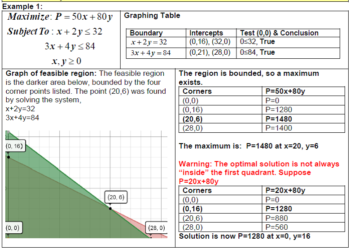
Example 1: Product Mix (Maximization)

A furniture company makes chairs and tables. Each chair earns $50 profit; each table earns $100. Assembling a chair takes 2 labor hours and 1 unit of wood. A table takes 3 labor hours and 1 unit of wood. The company has 100 labor hours and 30 units of wood available.

• Decision variables: $x_1$ = chairs produced, $x_2$ = tables produced
• Objective: Maximize $Z = 50x_1 + 100x_2$
• Constraints:
  • $2x_1 + 3x_2 \leq 100$ (labor hours)
  • $x_1 + x_2 \leq 30$ (wood units)
  • $x_1 \geq 0,\ x_2 \geq 0$

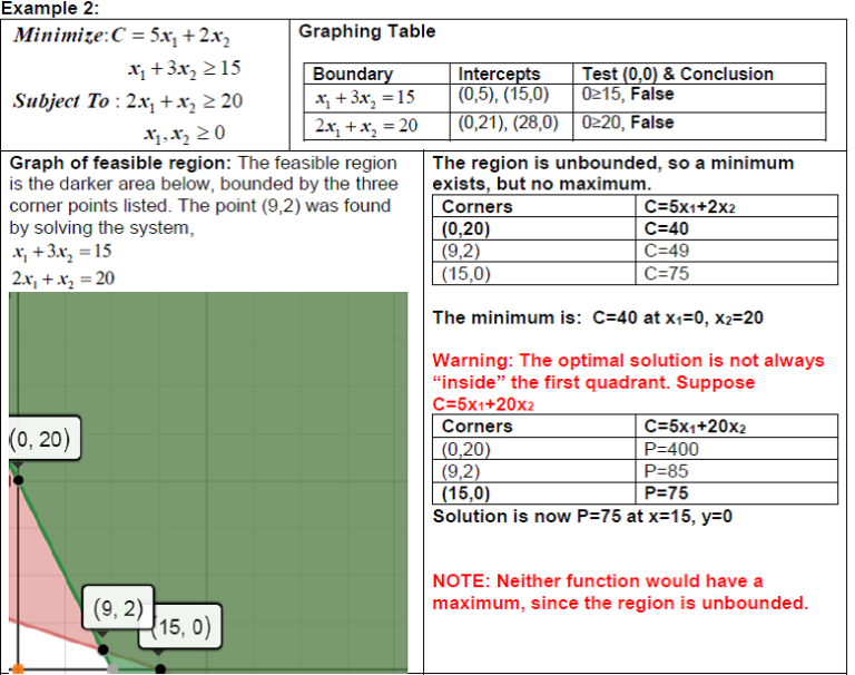
Example 2: Distribution (Minimization)

A company ships goods from multiple sources to multiple destinations. The goal is to minimize total shipping cost.

• Decision variables: $x_{ij}$ = units shipped from source $i$ to destination $j$
• Objective: Minimize $Z = \sum c_{ij} \cdot x_{ij}$, where $c_{ij}$ is the cost per unit shipped on that route
• Constraints: supply limits at each source, demand requirements at each destination, and non-negativity for all $x_{ij}$

Graphical Solutions for Linear Programs

Plotting Constraints and the Feasible Region

The graphical method works for LP problems with two decision variables. You plot everything on a standard x-y coordinate plane.

Here's how to build the graph step by step:

1. Convert each inequality to an equation and plot it as a straight line. For example, $x_1 + 2x_2 \leq 10$ becomes the line $x_1 + 2x_2 = 10$. Find two easy points (set $x_1 = 0$ to get $x_2 = 5$; set $x_2 = 0$ to get $x_1 = 10$) and draw the line.
2. Determine the feasible side of each line. Pick a test point (the origin works if it's not on the line). If the test point satisfies the inequality, shade toward it; otherwise, shade the opposite side.
3. Include the non-negativity constraints ($x_1 \geq 0$, $x_2 \geq 0$), which restrict the feasible region to the first quadrant.
4. Identify the feasible region as the area where all shaded regions overlap. This is typically a convex polygon.
5. Find all corner points (also called extreme points or vertices) by solving pairs of constraint equations simultaneously. These intersections are the candidates for the optimal solution.

Special Cases

Not every LP problem has a neat, bounded solution:

• Infeasible problem: The constraints contradict each other, so no point satisfies all of them at once. The feasible region is empty.
• Unbounded feasible region: The constraints don't fully enclose the region in every direction. For a maximization problem, this can mean the objective value can increase without limit (an unbounded solution). But an unbounded region doesn't always mean an unbounded solution; it depends on the direction of the objective function.
• Multiple optimal solutions: When the objective function line is parallel to one of the binding constraint edges, every point along that edge between two optimal corner points is equally optimal.

Optimal Solutions in Linear Programs

Finding the Optimal Solution

The Fundamental Theorem of Linear Programming guarantees that if an optimal solution exists, at least one will be found at a corner point of the feasible region. This gives you two methods:

Corner Point Method:

1. List all corner points of the feasible region (found by solving intersections of constraint lines).
2. Evaluate the objective function at each corner point.
3. For maximization, pick the corner point with the highest value. For minimization, pick the lowest.

Isoprofit (Iso-cost) Line Method:

1. Pick an arbitrary value for $Z$ and draw the line for the objective function (e.g., $3x_1 + 4x_2 = 12$).
2. Slide this line parallel to itself across the feasible region in the direction that improves $Z$ (outward for maximization, inward for minimization).
3. The last point (or edge) in the feasible region that the line touches is the optimal solution.

Example: Maximize $Z = 3x_1 + 4x_2$ with corner points at $(0, 0)$, $(6, 0)$, $(4, 3)$, and $(0, 5)$. Evaluate: $Z(0,0) = 0$, $Z(6,0) = 18$, $Z(4,3) = 24$, $Z(0,5) = 20$. The optimal solution is $(4, 3)$ with $Z^* = 24$.

Handling Special Cases

• Degeneracy occurs when more than two constraint lines intersect at a single corner point. This means one or more slack/surplus variables equal zero at that point. It can complicate algorithmic methods like the Simplex method, but it doesn't necessarily change the optimal value you find graphically.
• Unbounded solutions mean the objective function can improve indefinitely. This usually signals a modeling error (a missing constraint).
• No feasible solution means the constraints are contradictory. Check whether a constraint was set up incorrectly or if the problem truly has no solution.

Interpreting Graphical Solutions

Understanding Solution Components

Once you've found the optimal point, there's more to extract from the graph than just the answer:

• Optimal values of the decision variables tell you exactly how much of each product to make, ship, etc.
• Binding constraints are the ones that pass directly through the optimal point. These are the constraints that are "used up" completely (slack = 0). They're the active limits on your solution.
• Non-binding constraints have leftover capacity. The slack value for a non-binding "≤" constraint equals the difference between the right-hand side and the left-hand side evaluated at the optimal point. For example, if $x_1 + x_2 \leq 30$ and the optimal point gives $x_1 + x_2 = 25$, the slack is 5 units of unused wood.
• Shadow price (also called dual value) of a constraint is how much the objective function value improves per one-unit increase in that constraint's right-hand side. A binding constraint typically has a positive shadow price; a non-binding constraint has a shadow price of zero.

Sensitivity Analysis

Sensitivity analysis asks: how much can the problem data change before the current optimal solution changes?

• Range of optimality for an objective function coefficient: Rotate the objective function line around the current optimal corner point. The coefficient can change as long as the slope of the objective function stays between the slopes of the two binding constraints at that point. Beyond that range, a different corner point becomes optimal.
• Right-hand side changes: Increasing the right-hand side of a binding constraint shifts that constraint line outward, potentially expanding the feasible region and improving the objective value. The shadow price tells you the rate of improvement, but only within a limited range before the set of binding constraints changes.
• Graphical advantage: The visual nature of the graph makes it easier to see why a solution is optimal and how sensitive it is to changes. You can literally see the feasible region shift and the optimal point move.