7.1 One-Dimensional Steady-State Diffusion

Steady-State Diffusion in One Dimension

Steady-state diffusion describes how a chemical species moves from regions of high concentration to low concentration when the system has settled into a condition that no longer changes with time. Understanding this process is foundational for designing membranes, catalytic reactors, and separation systems where you need to predict mass transfer rates through simple geometries.

Concept and Characteristics

At steady state, the concentration at every point in the system stays constant over time. That doesn't mean nothing is moving. Species are still diffusing, but the rate of material entering any small volume element equals the rate leaving it. The result is a diffusive flux that is constant throughout the system.

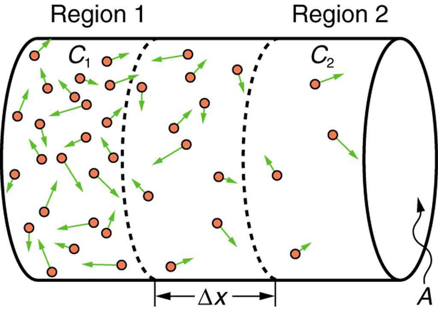
In the one-dimensional case, concentration and flux vary along only a single spatial coordinate (call it $x$). The other two directions ($y$ and $z$) are uniform. Practical examples include diffusion through a thin membrane or along a long, narrow tube.

Driving Force and Diffusion Direction

The driving force for diffusion is the concentration gradient, $\frac{dC}{dx}$, which measures the change in concentration per unit distance. Species always diffuse down the gradient, from high concentration toward low concentration.

This directionality follows from the second law of thermodynamics: systems evolve toward maximum entropy (or minimum Gibbs free energy). Diffusion continues until the gradient is eliminated and concentration becomes uniform everywhere.

Fick's First Law of Diffusion

Mathematical Expression

Fick's first law is the governing equation for steady-state diffusion. It states that the diffusive flux is proportional to the negative of the concentration gradient:

$J = -D\frac{dC}{dx}$

where:

• $J$ is the diffusive flux (mol/m²·s), the amount of species crossing a unit area per unit time
• $D$ is the diffusion coefficient (m²/s), a measure of how easily a species moves through a given medium
• $\frac{dC}{dx}$ is the concentration gradient (mol/m⁴)

The negative sign ensures that $J$ is positive when diffusion occurs in the direction of decreasing concentration (the positive $x$-direction if concentration decreases with $x$).

Diffusion Coefficient and Its Dependencies

The diffusion coefficient $D$ is not a universal constant; it depends on several factors:

• Temperature: Higher temperatures increase molecular kinetic energy, which generally raises $D$.
• Pressure: Pressure significantly affects diffusion in gases (higher pressure lowers $D$ because molecules are packed more tightly) but has minimal effect in liquids and solids.
• Molecular size and mass: Larger, heavier molecules diffuse more slowly, so they have smaller $D$ values.

Two common estimation methods:

• Stokes-Einstein equation (for liquids): Relates $D$ to temperature, solvent viscosity, and the hydrodynamic radius of the diffusing molecule. Useful for dilute solutions of roughly spherical solutes.
• Chapman-Enskog theory (for gases): Predicts $D$ from molecular weights, collision diameters, and intermolecular potential parameters of both species.

Concentration Profiles and Fluxes

Linear Concentration Profiles

Because the flux $J$ is constant at steady state and $D$ is typically treated as constant, Fick's first law requires $\frac{dC}{dx}$ to be constant as well. That means the concentration varies linearly with position:

$C(x) = C_1 + \frac{C_2 - C_1}{L}\,x$

where:

• $C_1$ is the concentration at $x = 0$
• $C_2$ is the concentration at $x = L$
• $L$ is the total thickness (or length) of the diffusion path

The slope of this line, $\frac{C_2 - C_1}{L}$, is the concentration gradient that drives diffusion.

Calculating Diffusive Fluxes

To find the flux through a slab or membrane of thickness $L$ with known boundary concentrations:

1. Determine the concentration gradient: $\frac{dC}{dx} = \frac{C_2 - C_1}{L}$

2. Look up or calculate the diffusion coefficient $D$ for the species-medium pair at the given conditions.

3. Substitute into Fick's first law:

$J = -D\frac{C_2 - C_1}{L}$

If $C_1 > C_2$, the gradient is negative and $J$ comes out positive, confirming diffusion in the positive $x$-direction. The magnitude of $J$ increases with a steeper gradient (larger $\Delta C$ or smaller $L$) and with a larger diffusion coefficient.

Boundary Conditions and Diffusion

Types of Boundary Conditions

Boundary conditions pin down the concentration profile by specifying what happens at the edges of the domain. Three standard types appear in diffusion problems:

1. Constant concentration (Dirichlet):

   • A fixed concentration is maintained at the boundary.
   • Produces the classic linear profile across the domain.
   • Example: a gas-liquid interface where the liquid surface stays saturated with the dissolved gas.

2. Constant flux (Neumann):

   • A fixed diffusive flux is imposed at the boundary.
   • The concentration profile still has a constant slope, but the absolute concentration values shift to satisfy the flux condition.
   • Example: a catalytic surface consuming a reactant at a known, constant rate.

3. Mixed (Robin):

   • Combines concentration and flux through a mass transfer coefficient: the flux at the boundary is proportional to the difference between the surface concentration and some external value.
   • Example: a porous membrane where external convective resistance affects the surface concentration.

Effects of Boundary Conditions on Diffusion

Certain special boundaries simplify the math considerably:

• Impermeable boundaries impose a zero-flux condition ($J = 0$), meaning nothing passes through. At that boundary, $\frac{dC}{dx} = 0$.
• Symmetry planes let you analyze only half the domain, since the concentration profile mirrors itself across the plane.

Changing boundary values has a direct, predictable effect on the solution:

• Increasing the concentration difference $\Delta C$ between the two boundaries steepens the gradient and raises the flux proportionally.
• Decreasing $\Delta C$ flattens the profile and reduces the flux.

For more complex geometries or boundary combinations, techniques like integration of the governing ODE (which, at steady state in 1-D, is simply $\frac{d^2C}{dx^2} = 0$) with the applied boundary conditions will yield the concentration profile and flux. These results are directly applicable to designing separation membranes, sizing catalytic pellets, and predicting transport rates in heat and mass transfer equipment.