4.2 Monopole antennas

Monopole antenna basics

A monopole antenna is a single radiating element mounted perpendicular to a conducting ground plane. By exploiting image theory, this half-structure reproduces the fields of a full dipole in the upper half-space while being physically half the size. That combination of compact geometry and omnidirectional azimuthal coverage makes the monopole one of the most widely deployed antenna types in practice.

Monopole vs dipole antennas

A dipole antenna has two symmetrical arms fed at the center, and it radiates into the full sphere. A monopole keeps only one arm and replaces the missing half with a ground plane. Image theory tells you why this works: a perfect ground plane creates a virtual mirror image of the monopole element, so the fields above the plane are identical to those of a dipole.

Key differences:

• A monopole is half the physical length of the equivalent dipole ($\lambda/4$ vs $\lambda/2$).
• The monopole's input impedance is half that of the corresponding dipole because it radiates into only the upper hemisphere.
• The monopole's directivity is about 3 dB higher than the equivalent dipole's, since all radiated power is concentrated above the ground plane.

Monopole antenna structure

A monopole antenna has three main parts:

• Radiating element: a straight conductor (wire, rod, or printed trace) oriented perpendicular to the ground plane. For the standard quarter-wave monopole, its length is $L = \lambda/4$.
• Ground plane: a flat conducting surface at the base. It can be a physical metal sheet, a set of radial wires, or a PCB copper pour. The ground plane must be large enough (ideally infinite, practically at least $\lambda/4$ radius) to approximate the image well.
• Feed point: located at the junction of the radiating element and the ground plane, where the transmission line connects.

Current distribution of monopoles

The current along a quarter-wave monopole follows a sinusoidal profile:

• Maximum current at the feed point (base of the element).
• Current tapers as $I(z) = I_0 \cos(kz)$, where $k = 2\pi/\lambda$ and $z$ is the distance from the base.
• Zero current at the tip of the element (open-circuit boundary condition).

This distribution directly determines both the radiation pattern and the input impedance. A longer monopole (e.g., $5\lambda/8$) shifts the current distribution and changes the pattern shape, sometimes producing a lower-angle main lobe at the cost of introducing sidelobes.

Impedance of monopole antennas

Because the monopole radiates into a half-space, its input impedance is half that of the equivalent dipole. For a thin quarter-wave monopole over a perfect ground plane:

$Z_{\text{in}} \approx 36.5 + j21.25 \;\Omega$

This is exactly half the dipole value of roughly $73 + j42.5 \;\Omega$. The reactive part ($j21.25\;\Omega$) tells you the antenna is slightly shorter than true resonance. Making the element a few percent longer than $\lambda/4$ can cancel the reactance and bring the input to nearly pure $36.5\;\Omega$ resistive.

Since most systems use $50\;\Omega$ transmission lines, a matching network is usually needed. Common options include an L-section LC network, a series stub, or a quarter-wave transformer.

Monopole antenna radiation

The radiation behavior of a monopole is shaped by two facts: the element is vertically polarized, and the ground plane confines radiation to the upper hemisphere. Together these produce the characteristic omnidirectional azimuthal pattern that makes monopoles so useful.

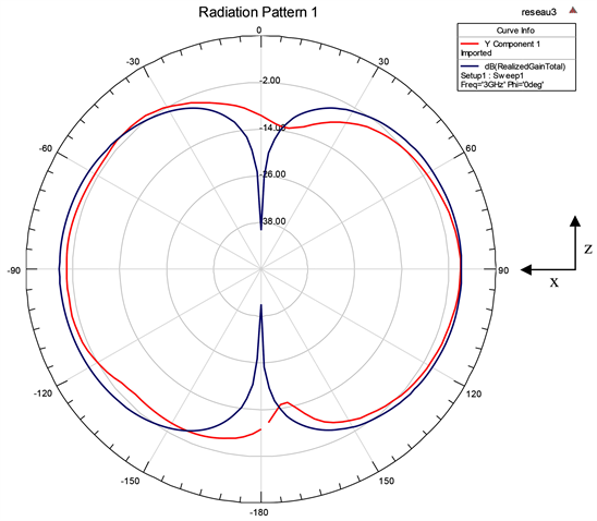
Radiation pattern of monopoles

• Horizontal (azimuthal) plane: The pattern is omnidirectional, meaning equal radiation in all directions around the antenna axis.
• Vertical (elevation) plane: The pattern has a single lobe that peaks at the horizon ($\theta = 90°$) and a null straight up ($\theta = 0°$, the zenith). For an ideal quarter-wave monopole over a perfect ground plane, the elevation pattern follows $E(\theta) \propto \frac{\cos\!\bigl(\frac{\pi}{2}\cos\theta\bigr)}{\sin\theta}$.

A finite or imperfect ground plane tilts the main lobe slightly upward and introduces ripple in the pattern. Radial ground wires or a larger ground plane help push the lobe back toward the horizon.

Directivity of monopole antennas

Directivity measures how strongly an antenna focuses power in its peak direction compared to an isotropic radiator. For a quarter-wave monopole over a perfect infinite ground plane:

$D \approx 5.17 \;\text{(linear)} = 7.14\;\text{dBi}$

This is exactly twice (3 dB more than) the directivity of a half-wave dipole ($D \approx 2.15\;\text{dBi}$), because the monopole concentrates the same pattern into only the upper hemisphere.

Gain of monopole antennas

Gain equals directivity multiplied by radiation efficiency ($G = \eta \cdot D$). For a lossless quarter-wave monopole over a perfect ground plane, gain equals directivity: roughly 5.17 (linear) or 7.14 dBi.

In practice, gain is reduced by:

• Finite ground plane size and shape
• Ohmic losses in the conductor and ground system
• Nearby lossy objects or structures
• Imperfect ground conductivity (especially relevant for AM broadcast towers over soil)

Real-world quarter-wave monopoles on modest ground planes typically achieve 2 to 5 dBi, depending on the ground plane quality.

Radiation resistance of monopoles

Radiation resistance is the equivalent resistance that accounts for the power actually radiated by the antenna. For a thin quarter-wave monopole over a perfect ground plane:

$R_{\text{rad}} \approx 36.5\;\Omega$

This is half the radiation resistance of a half-wave dipole ($\approx 73\;\Omega$). Radiation resistance matters for efficiency: the antenna's radiation efficiency is

$\eta = \frac{R_{\text{rad}}}{R_{\text{rad}} + R_{\text{loss}}}$

A higher radiation resistance relative to loss resistance means better efficiency. Short monopoles ($L \ll \lambda/4$) have very low radiation resistance, making them prone to poor efficiency unless losses are carefully minimized.

Monopole antenna types

Several monopole variants address practical constraints like size, bandwidth, and impedance matching. Each modifies the basic quarter-wave design in a specific way.

Quarter-wave monopole antennas

The quarter-wave monopole is the baseline design: a straight conductor of length $L = \lambda/4$ over a ground plane. Its advantages are simplicity and predictable performance. At 2.4 GHz (Wi-Fi), for example, $\lambda/4 \approx 31\;\text{mm}$, which fits easily on a wireless router. At 1 MHz (AM broadcast), $\lambda/4 \approx 75\;\text{m}$, requiring a tall tower.

Folded monopole antennas

A folded monopole bends the radiating element back toward the ground plane, forming a closed loop. This has two main effects:

• Higher input impedance: roughly four times that of a simple monopole ($\approx 150\;\Omega$), which can simplify matching to certain feed lines.
• Wider bandwidth: the folded geometry introduces a transmission-line mode in addition to the antenna mode, broadening the impedance bandwidth.

Folded monopoles appear in mobile handsets and compact base station antennas where bandwidth is a priority.

Top-loaded monopole antennas

Top-loading adds a capacitive structure (a disk, hat, or set of radial wires) at the tip of the monopole. This forces the current distribution to remain more uniform along the element, which:

• Allows the antenna to be physically shorter than $\lambda/4$ while maintaining reasonable radiation resistance.
• Improves efficiency compared to a simple shortened monopole of the same height.

AM broadcast antennas and portable HF/VHF radios frequently use top-loading to keep antenna height manageable.

Sleeve monopole antennas

A sleeve monopole surrounds the lower portion of the radiating element with a coaxial conducting cylinder. The sleeve acts as an integrated impedance transformer, providing:

• Broader bandwidth than a plain monopole (often 2:1 or wider frequency ratio).
• A more stable radiation pattern across the operating band.

Sleeve monopoles are common in vehicular and base station antennas where wideband operation is required.

Monopole antenna applications

Monopoles in wireless communications

Monopole antennas serve as the workhorse for many wireless standards. Base station sector antennas often use arrays of monopole-derived elements. On the user side, Wi-Fi access points at 2.4 GHz and 5 GHz commonly use quarter-wave monopoles (or variants) because omnidirectional coverage and small size are both needed. Cellular systems operating at bands like 700 MHz, 1.8 GHz, or 3.5 GHz also rely on monopole-type elements integrated into handsets and small cells.

Monopoles for AM broadcasting

AM broadcast stations (530 to 1700 kHz) typically use tall monopole towers as their primary radiating element. At 1 MHz, a quarter-wave monopole is about 75 m tall. The ground system consists of a network of buried radial wires extending at least $\lambda/4$ from the tower base to approximate a good ground plane over lossy soil. Directional AM stations use arrays of monopole towers with controlled phasing to shape coverage and protect other stations.

Monopoles in mobile devices

Modern smartphones rarely use a simple wire monopole, but the underlying principle persists. Planar inverted-F antennas (PIFAs) and other compact structures used in phones are derived from the monopole concept, with the ground plane provided by the device's PCB. These antennas are designed to cover multiple bands (e.g., 700 MHz LTE, 2.4 GHz Wi-Fi, 1.575 GHz GPS) in a volume of just a few cubic centimeters.

Monopoles for IoT devices

IoT devices such as sensors, smart home hubs, and wearables need antennas that are small, cheap, and power-efficient. Printed monopoles on PCB substrates are a popular choice for protocols like Zigbee (2.4 GHz), LoRa (sub-GHz, e.g., 868 MHz or 915 MHz), and NB-IoT. A quarter-wave monopole at 915 MHz is about 82 mm, which can be meandered or folded to fit within a compact enclosure.

Monopole antenna design

Monopole length vs frequency

The fundamental design equation for a quarter-wave monopole is:

$L = \frac{c}{4f} = \frac{\lambda}{4}$

where $c \approx 3 \times 10^8\;\text{m/s}$ is the speed of light and $f$ is the operating frequency.

Example: For a 900 MHz GSM antenna, $L = \frac{3 \times 10^8}{4 \times 900 \times 10^6} \approx 83\;\text{mm}$.

In practice, the physical length is slightly shorter than the free-space calculation because of the finite diameter of the element and fringing effects. A typical correction factor is 0.95 to 0.97, so you'd trim the element to around 79 to 81 mm and fine-tune experimentally or in simulation.

Monopole diameter considerations

The element's diameter (or width, for a printed trace) affects performance in several ways:

• Bandwidth: Thicker elements have lower Q and therefore wider impedance bandwidth. A monopole with diameter $d = 0.01\lambda$ might have a 5% bandwidth, while $d = 0.05\lambda$ could reach 15% or more.
• Input impedance: Increasing diameter slightly lowers the resonant resistance and reduces the reactive component.
• Mechanical robustness: Thicker elements are sturdier, which matters for outdoor or vehicular antennas.

The trade-off is physical size. In PCB designs, trace width is constrained by board area.

Monopole feeding techniques

Three common feeding methods:

1. Coaxial feed: The inner conductor of a coaxial cable connects to the monopole element; the outer conductor connects to the ground plane. This is the most common method and provides a clean, well-defined feed point.
2. Direct (probe) feed: The monopole is soldered or connected directly to a signal trace, with the ground plane on the opposite side of the substrate. Simple but can introduce parasitic reactance.
3. Microstrip feed: A microstrip transmission line on a PCB transitions into the monopole element. This is convenient for integrated designs where the antenna shares a board with RF circuitry.

Each method introduces its own parasitic effects, so the matching network design should account for the specific feed topology.

Monopole matching networks

Since the quarter-wave monopole's input impedance ($\approx 36.5\;\Omega$ resistive at resonance) doesn't perfectly match a $50\;\Omega$ line, a matching network improves power transfer. The steps for designing a match:

1. Measure or simulate the antenna's complex impedance at the operating frequency.

2. Choose a matching topology. Common choices:

   • L-network (one inductor + one capacitor): simple, narrowband.
   • Quarter-wave transformer: a transmission line section of impedance $Z_T = \sqrt{Z_{\text{in}} \cdot Z_0}$ and length $\lambda/4$.
   • Stub matching: an open or shorted transmission line stub placed at a calculated distance from the feed.

3. Calculate component values or line dimensions using a Smith chart or matching network equations.

4. Verify with simulation or VNA measurement, and iterate as needed.

For wideband applications, multi-section or tapered matching networks may be necessary.

Monopole antenna arrays

Arranging multiple monopole elements into an array lets you shape the radiation pattern, increase gain, or steer the beam electronically. The array factor multiplies the single-element pattern to produce the total pattern.

Linear monopole arrays

A linear array places $N$ monopole elements along a straight line with uniform spacing $d$. The array factor for uniform spacing and progressive phase shift $\alpha$ is:

$AF(\theta) = \sum_{n=0}^{N-1} e^{\,jn(kd\cos\theta + \alpha)}$

• Broadside array ($\alpha = 0$, $d = \lambda/2$): the main beam points perpendicular to the array axis.
• End-fire array ($\alpha = -kd$): the main beam points along the array axis.

Increasing $N$ narrows the beamwidth and raises the directivity.

Planar monopole arrays

A planar array arranges monopole elements in a 2D grid (e.g., $M \times N$). This provides beam control in both azimuth and elevation. The total array factor is the product of the row and column array factors. Planar arrays can produce pencil beams (narrow in both planes), fan beams, or shaped patterns depending on the amplitude and phase weights applied to each element.

Phased monopole arrays

In a phased array, each element's feed signal has an independently controllable phase (and sometimes amplitude). By adjusting these phases electronically, you steer the beam without physically moving the antenna. The required phase shift for steering to angle $\theta_0$ in a linear array is:

$\alpha = -kd\sin\theta_0$

Phased arrays are central to modern radar, satellite communications, and 5G millimeter-wave systems, where rapid beam switching is essential.

Beam steering with monopole arrays

Beam steering with a monopole array follows this process:

1. Define the desired beam direction $(\theta_0, \phi_0)$.
2. Calculate the required phase shift for each element based on its position and the target direction.
3. Apply these phase shifts using electronic phase shifters (analog or digital) at each element's feed.
4. The array factor shifts its main lobe to the desired direction while the element pattern (the individual monopole's pattern) acts as an envelope.

Practical considerations include grating lobes (which appear when $d > \lambda/2$), scan blindness at certain angles, and mutual coupling between elements, which alters each element's impedance and pattern.

Monopole antenna measurements

Verifying antenna performance through measurement is a critical part of the design cycle. The four key quantities to measure are impedance, radiation pattern, gain, and bandwidth.

Measuring monopole impedance

A vector network analyzer (VNA) is the standard instrument for impedance measurement. The procedure:

1. Calibrate the VNA at the reference plane (the antenna's feed point) using known standards (open, short, load).
2. Connect the monopole antenna to the VNA port.
3. Measure the reflection coefficient $S_{11}$ over the frequency range of interest.
4. The VNA converts $S_{11}$ to input impedance: $Z_{\text{in}} = Z_0 \frac{1 + S_{11}}{1 - S_{11}}$.

Plot $S_{11}$ on a Smith chart to visualize the impedance trajectory and identify the resonant frequency (where the imaginary part crosses zero).

Measuring monopole radiation patterns

Radiation pattern measurements are typically performed in an anechoic chamber to eliminate reflections. The process:

1. Mount the monopole (with its ground plane) on a positioner that can rotate in azimuth and elevation.
2. Place a known reference antenna (the "source") at a fixed position, far enough away to be in the far field ($R > 2D^2/\lambda$, where $D$ is the largest antenna dimension).
3. Transmit a CW signal from the source and record the received power at the monopole as the positioner sweeps through angles.
4. Normalize the data to the peak value to obtain the relative radiation pattern.

From the measured pattern, you can extract beamwidth, sidelobe levels, null locations, and front-to-back ratio.

Measuring monopole gain

Two standard methods for gain measurement:

• Gain-transfer (substitution) method: Replace the antenna under test with a calibrated reference antenna (known gain). The difference in received power gives the gain of the test antenna relative to the reference.
• Two-antenna method: Use two identical antennas facing each other. Measure the received power and apply the Friis transmission equation to extract the gain of each antenna.

Both methods require far-field conditions and a well-controlled measurement environment.

Measuring monopole bandwidth

Bandwidth is most commonly defined by the $S_{11} < -10\;\text{dB}$ criterion (corresponding to a VSWR < 2:1, meaning less than 11% of power is reflected).

1. Sweep $S_{11}$ across frequency using a VNA.
2. Identify the lower frequency $f_L$ and upper frequency $f_U$ where $S_{11} = -10\;\text{dB}$.
3. The impedance bandwidth is $BW = f_U - f_L$, or as a percentage: $\%BW = \frac{f_U - f_L}{f_0} \times 100$, where $f_0$ is the center frequency.

A typical thin quarter-wave monopole has about 5 to 10% impedance bandwidth. Thicker elements, folded designs, or sleeve configurations extend this significantly.