5.2 Relativistic electrodynamics

Relativistic electrodynamics merges electromagnetic theory with special relativity, revealing that electric and magnetic fields are not independent entities but different aspects of a single electromagnetic field. How that field appears depends on your reference frame. This topic covers how fields transform between frames, the tensor machinery that keeps Maxwell's equations frame-independent, and the radiation produced by relativistic charges.

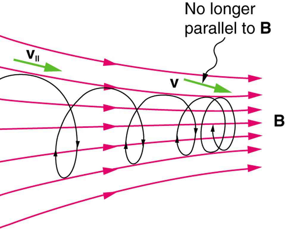
Lorentz transformations of fields

When you boost from one inertial frame to another, the electric and magnetic fields mix together. A pure electric field in one frame can have a magnetic component in another, and vice versa. The transformation rules follow directly from the postulates of special relativity: the laws of physics are the same in all inertial frames, and the speed of light is invariant.

Electric field transformations

The components of $\vec{E}$ parallel to the boost velocity $\vec{v}$ are unchanged:

$E_{\parallel}' = E_{\parallel}$

The perpendicular components pick up a contribution from the magnetic field:

$\vec{E}_{\perp}' = \gamma(\vec{E}_{\perp} + \vec{v} \times \vec{B})$

where $\gamma = 1/\sqrt{1 - v^2/c^2}$ is the Lorentz factor. The appearance of $\vec{B}$ in the transformation of $\vec{E}$ is the clearest sign that electric and magnetic fields are frame-dependent projections of a single object.

Magnetic field transformations

The same pattern holds for $\vec{B}$. Parallel components are invariant:

$B_{\parallel}' = B_{\parallel}$

Perpendicular components mix in the electric field:

$\vec{B}_{\perp}' = \gamma\left(\vec{B}_{\perp} - \frac{\vec{v} \times \vec{E}}{c^2}\right)$

Notice the symmetry: $\vec{E}$ transforms with $+\vec{v} \times \vec{B}$, while $\vec{B}$ transforms with $-\vec{v} \times \vec{E}/c^2$. The factor of $1/c^2$ reflects the difference in SI units between electric and magnetic fields.

Field tensor

The electromagnetic field tensor $F^{\mu\nu}$ packages all six field components (three from $\vec{E}$, three from $\vec{B}$) into a single 4×4 antisymmetric matrix. Antisymmetry ($F^{\mu\nu} = -F^{\nu\mu}$) means the diagonal is zero and there are exactly six independent entries, matching the six field components.

Under a Lorentz boost $\Lambda$, the tensor transforms as:

$F'^{\mu\nu} = \Lambda^{\mu}_{\ \alpha}\,\Lambda^{\nu}_{\ \beta}\,F^{\alpha\beta}$

This single rule reproduces all the component-by-component transformation formulas above. The field tensor also makes it straightforward to identify Lorentz invariants of the electromagnetic field:

• $F_{\mu\nu}F^{\mu\nu} = 2(B^2 - E^2/c^2)$
• $\frac{1}{2}\epsilon_{\mu\nu\alpha\beta}F^{\mu\nu}F^{\alpha\beta} = -\frac{4}{c}\,\vec{E}\cdot\vec{B}$

These two quantities have the same value in every inertial frame.

Covariant formulation of electrodynamics

The covariant formulation rewrites all of electrodynamics using four-vectors and tensors so that Lorentz invariance is manifest. You never have to check frame-independence equation by equation; it's built into the notation.

Four-current density

Charge density $\rho$ and current density $\vec{J}$ combine into the four-current:

$J^{\mu} = (\rho c,\, \vec{J})$

Because $J^{\mu}$ is a four-vector, it transforms properly under boosts. Charge conservation takes the compact form:

$\partial_{\mu} J^{\mu} = 0$

This is the continuity equation $\partial \rho/\partial t + \nabla \cdot \vec{J} = 0$ written in manifestly covariant language.

Electromagnetic field tensor

The explicit matrix form of $F^{\mu\nu}$ (in SI, with signature $+{-}{-}{-}$) is:

$F^{\mu\nu} = \begin{pmatrix} 0 & -E_x/c & -E_y/c & -E_z/c \\ E_x/c & 0 & -B_z & B_y \\ E_y/c & B_z & 0 & -B_x \\ E_z/c & -B_y & B_x & 0 \end{pmatrix}$

The six independent components split into the electric field (the $0i$ components) and the magnetic field (the $ij$ components). The dual tensor $\tilde{F}^{\mu\nu} = \frac{1}{2}\epsilon^{\mu\nu\alpha\beta}F_{\alpha\beta}$ swaps the roles of $\vec{E}$ and $\vec{B}$.

Covariant form of Maxwell's equations

All four of Maxwell's equations reduce to two tensor equations:

1. Inhomogeneous equations (Gauss's law + Ampère-Maxwell law):

$\partial_{\mu} F^{\mu\nu} = \mu_0 J^{\nu}$

1. Homogeneous equations (Faraday's law + no magnetic monopoles), expressed via the Bianchi identity:

$\partial_{\lambda} F_{\mu\nu} + \partial_{\mu} F_{\nu\lambda} + \partial_{\nu} F_{\lambda\mu} = 0$

Equivalently, using the dual tensor: $\partial_{\mu}\tilde{F}^{\mu\nu} = 0$.

Lorentz invariance

Because both equations above are written entirely in terms of tensors contracted with four-derivatives, they automatically hold in every inertial frame. You don't need to re-derive anything when you boost. This is the payoff of the covariant formulation: the form of the equations is the same for all inertial observers.

Relativistic charged particle dynamics

At speeds approaching $c$, the Newtonian equation $\vec{F} = m\vec{a}$ breaks down. You need relativistic momentum, and the relationship between force and acceleration becomes velocity-dependent.

Equation of motion in electromagnetic fields

The relativistic Lorentz force law is:

$\frac{d\vec{p}}{dt} = q(\vec{E} + \vec{v} \times \vec{B})$

where $\vec{p} = \gamma m \vec{v}$ is the relativistic momentum. The force on the right side looks identical to the non-relativistic expression, but the left side now involves $\gamma$, which makes the effective inertia increase with speed.

In covariant form, this becomes:

$\frac{dp^{\mu}}{d\tau} = q F^{\mu\nu} u_{\nu}$

where $p^{\mu} = m u^{\mu}$ is the four-momentum, $u^{\mu}$ is the four-velocity, and $\tau$ is proper time.

Relativistic momentum and energy

• Relativistic momentum: $\vec{p} = \gamma m \vec{v}$
• Total energy: $E = \gamma mc^2$, which includes rest energy $mc^2$ plus kinetic energy $(\gamma - 1)mc^2$
• Energy-momentum relation: $E^2 = p^2c^2 + m^2c^4$

This last relation is frame-independent and holds even for massless particles (photons), where $E = pc$.

Covariant Lagrangian formulation

The action for a relativistic charged particle in an electromagnetic field is:

$S = \int \left(-mc^2\sqrt{1 - v^2/c^2} + q\vec{v}\cdot\vec{A} - q\phi\right) dt$

The Lagrangian is therefore:

$L = -mc^2\sqrt{1 - v^2/c^2} + q\vec{v}\cdot\vec{A} - q\phi$

where $\phi$ is the scalar potential and $\vec{A}$ is the vector potential. Applying the Euler-Lagrange equations to this Lagrangian reproduces the relativistic Lorentz force equation. In manifestly covariant form, the action can be written as:

$S = \int \left(-mc\,ds + qA_{\mu}\,dx^{\mu}\right)$

where $ds = c\,d\tau$ is the invariant interval.

Electromagnetic stress-energy tensor

The stress-energy tensor $T^{\mu\nu}$ encodes everything about the energy and momentum content of the electromagnetic field. It's a symmetric 4×4 tensor defined by:

$T^{\mu\nu} = \frac{1}{\mu_0}\left(F^{\mu\alpha}F^{\nu}_{\ \alpha} - \frac{1}{4}\eta^{\mu\nu}F_{\alpha\beta}F^{\alpha\beta}\right)$

where $\eta^{\mu\nu}$ is the Minkowski metric.

Energy density and Poynting vector

The $T^{00}$ component gives the electromagnetic energy density:

$u = \frac{1}{2}\left(\varepsilon_0 E^2 + \frac{B^2}{\mu_0}\right)$

The $T^{0i}$ components (divided by $c$) give the Poynting vector:

$\vec{S} = \frac{1}{\mu_0}\vec{E}\times\vec{B}$

which describes the rate and direction of energy flow per unit area.

Momentum density and Maxwell stress tensor

The momentum density of the field is:

$\vec{g} = \frac{\vec{S}}{c^2} = \varepsilon_0(\vec{E}\times\vec{B})$

Note that $\vec{g} = \vec{S}/c^2$, consistent with the relativistic relation between energy flux and momentum density.

The spatial components $T^{ij}$ form the Maxwell stress tensor $\sigma_{ij}$, which gives the flux of the $i$-th component of momentum through a surface with normal in the $j$-direction. It's the tool you use to calculate electromagnetic forces on surfaces.

Conservation laws

Energy-momentum conservation for the electromagnetic field is:

$\partial_{\mu} T^{\mu\nu} = -F^{\nu\alpha}J_{\alpha}$

The right side is the rate at which the field does work on charges and transfers momentum to them. In a region with no charges, this reduces to $\partial_{\mu} T^{\mu\nu} = 0$, which encodes both Poynting's theorem ($\nu = 0$) and conservation of field momentum ($\nu = i$).

The symmetry of $T^{\mu\nu}$ ($T^{\mu\nu} = T^{\nu\mu}$) is connected to conservation of angular momentum.

Relativistic potentials and gauge invariance

Four-potential

The scalar and vector potentials combine into the four-potential:

$A^{\mu} = (\phi/c,\, \vec{A})$

The field tensor is then:

$F^{\mu\nu} = \partial^{\mu}A^{\nu} - \partial^{\nu}A^{\mu}$

This definition automatically satisfies the homogeneous Maxwell equations (the Bianchi identity), so you only need to solve the inhomogeneous ones.

Gauge invariance

The physical fields $F^{\mu\nu}$ are unchanged under a gauge transformation:

$A^{\mu} \to A^{\mu} + \partial^{\mu}\chi$

for any scalar function $\chi(x)$. This means the potentials contain redundant degrees of freedom. You can exploit this freedom by choosing a gauge condition that simplifies your calculation.

Lorentz gauge condition

The Lorentz gauge (also called Lorenz gauge, after Ludvig Lorenz) imposes:

$\partial_{\mu}A^{\mu} = 0$

This condition is itself Lorentz-covariant, which makes it the natural choice for relativistic problems. It decouples the equations for the four components of $A^{\mu}$.

Inhomogeneous wave equations

In the Lorentz gauge, each component of the four-potential satisfies:

$\square A^{\mu} = \mu_0 J^{\mu}$

where $\square = \partial_{\mu}\partial^{\mu} = \frac{1}{c^2}\frac{\partial^2}{\partial t^2} - \nabla^2$ is the d'Alembertian operator. All four components obey the same type of wave equation, just with different source terms.

Retarded potentials

The physical (causal) solution to the wave equation is the retarded potential:

$A^{\mu}(\vec{r}, t) = \frac{\mu_0}{4\pi}\int \frac{J^{\mu}(\vec{r}', t_r)}{|\vec{r} - \vec{r}'|}\,d^3r'$

where $t_r = t - |\vec{r} - \vec{r}'|/c$ is the retarded time. The source is evaluated at the earlier time when a light signal would have had to leave $\vec{r}'$ to arrive at $\vec{r}$ at time $t$. This enforces causality: fields at a point depend only on what happened in its past light cone.

Radiation from moving charges

Accelerating charges radiate. At relativistic speeds, the radiation pattern becomes highly directional and the radiated power increases dramatically.

Liénard-Wiechert potentials

For a single point charge $q$ moving along a trajectory $\vec{w}(t)$, the retarded potentials take a specific form called the Liénard-Wiechert potentials:

$\phi(\vec{r}, t) = \frac{q}{4\pi\varepsilon_0}\frac{1}{R(1 - \hat{R}\cdot\vec{\beta})}\bigg|_{t_r}$

$\vec{A}(\vec{r}, t) = \frac{\mu_0 q c}{4\pi}\frac{\vec{\beta}}{R(1 - \hat{R}\cdot\vec{\beta})}\bigg|_{t_r}$

Here $\vec{R} = \vec{r} - \vec{w}(t_r)$ is the vector from the retarded position to the field point, $R = |\vec{R}|$, $\hat{R} = \vec{R}/R$, and $\vec{\beta} = \vec{v}/c$. Everything on the right is evaluated at the retarded time $t_r$.

The factor $1/(1 - \hat{R}\cdot\vec{\beta})$ is crucial. It causes the potentials (and fields) to be strongly enhanced in the forward direction when $\vec{\beta}$ is close to $\hat{R}$, i.e., when the charge is moving toward the observer at nearly the speed of light.

Fields of a relativistic point charge

Differentiating the Liénard-Wiechert potentials gives the electric field, which splits into two terms:

$\vec{E} = \frac{q}{4\pi\varepsilon_0}\left[\frac{(\hat{R} - \vec{\beta})(1 - \beta^2)}{(1 - \hat{R}\cdot\vec{\beta})^3 R^2} + \frac{\hat{R}\times\left[(\hat{R} - \vec{\beta})\times\dot{\vec{\beta}}\right]}{c(1 - \hat{R}\cdot\vec{\beta})^3 R}\right]_{t_r}$

• The first term (velocity field) falls off as $1/R^2$. It's the relativistic generalization of the Coulomb field and carries no energy to infinity.
• The second term (acceleration field) falls off as $1/R$. This is the radiation field, and it's the only part that contributes to radiated power at large distances.

The magnetic field is always:

$\vec{B} = \frac{\hat{R}}{c}\times\vec{E}$

so $\vec{B}$ is perpendicular to both $\hat{R}$ and $\vec{E}$, and $|\vec{B}| = |\vec{E}|/c$ for the radiation part.

Relativistic generalization of Larmor's formula

The total radiated power from an accelerating charge, valid at any speed, is:

$P = \frac{q^2}{6\pi\varepsilon_0 c}\gamma^6\left(\dot{\beta}^2 - |\vec{\beta}\times\dot{\vec{\beta}}|^2\right)$

The $\gamma^6$ factor is what makes synchrotron radiation so intense. Two important special cases:

• Acceleration parallel to velocity (linear accelerator): $P = \frac{q^2}{6\pi\varepsilon_0 c}\gamma^6\dot{\beta}^2$
• Acceleration perpendicular to velocity (circular orbit): $P = \frac{q^2}{6\pi\varepsilon_0 c}\gamma^4\dot{\beta}^2$

The perpendicular case has $\gamma^4$ instead of $\gamma^6$ because $|\vec{\beta}\times\dot{\vec{\beta}}|^2$ partially cancels $\dot{\beta}^2$. Even so, the $\gamma^4$ dependence means synchrotron losses scale as $E^4/m^4$, which is why electron synchrotrons lose far more energy to radiation than proton synchrotrons at the same energy.

Angular distribution of radiation

For a non-relativistic charge, radiation is emitted in the familiar dipole pattern (doughnut shape, with no radiation along the acceleration axis). As the speed increases, relativistic beaming compresses the radiation into a narrow forward cone.

The half-angle of this cone is approximately:

$\theta \sim \frac{1}{\gamma}$

For a 1 GeV electron ($\gamma \approx 2000$), the radiation cone has a half-angle of about 0.03°. The angular power distribution is:

$\frac{dP}{d\Omega} = \frac{q^2}{16\pi^2\varepsilon_0 c}\frac{\left|\hat{R}\times\left[(\hat{R} - \vec{\beta})\times\dot{\vec{\beta}}\right]\right|^2}{(1 - \hat{R}\cdot\vec{\beta})^5}$

The $(1 - \hat{R}\cdot\vec{\beta})^5$ in the denominator is what produces the extreme forward peaking.

Covariant Green functions

Green functions are the bridge between sources and fields. If you know the Green function for the wave equation, you can find the potential produced by any source distribution through a convolution integral.

Invariant delta function

The four-dimensional Dirac delta function $\delta^4(x - x')$ localizes a source to a single spacetime event. It satisfies:

$\int \delta^4(x - x') f(x')\,d^4x' = f(x)$

Under Lorentz transformations, $\delta^4(x - x')$ transforms as a scalar density (it picks up the Jacobian of the transformation, which is unity for proper Lorentz transformations). This ensures that integrals involving $\delta^4$ remain covariant.

Retarded Green function

The retarded Green function $G_R(x - x')$ solves:

$\square\, G_R(x - x') = \delta^4(x - x')$

with the boundary condition that $G_R = 0$ when $x^0 < x'^0$ (no effect before the cause). The explicit form is:

$G_R(x - x') = -\frac{1}{2\pi}\theta(x^0 - x'^0)\,\delta\!\left[(x - x')^2\right]$

where $(x - x')^2 = (x^0 - x'^0)^2 - |\vec{x} - \vec{x}'|^2$ is the spacetime interval and $\theta$ is the Heaviside step function. The delta function restricts contributions to the light cone, and the step function selects only the past light cone. This is the mathematical expression of causality and the finite speed of light.

The general retarded solution for the four-potential is then:

$A^{\mu}(x) = \mu_0 \int G_R(x - x')\,J^{\mu}(x')\,d^4x'$

which reproduces the retarded potential formula when the integration over $x'^0$ is carried out.