9.6 Hypothesis Testing of a Single Mean and Single Proportion

Hypothesis Testing for a Single Mean and Proportion

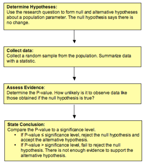
Hypothesis testing gives you a structured way to answer the question: does my sample data provide enough evidence to challenge a claim about a population? That "claim" is your null hypothesis, and the entire process revolves around deciding whether to reject it or not.

This section covers how to set up hypotheses, calculate the right test statistic, and interpret your results using p-values and significance levels.

Formulation of Hypotheses

Every hypothesis test starts with two competing statements about a population parameter (either a mean $\mu$ or a proportion $p$).

Null hypothesis ($H_0$): This is the "nothing special is happening" claim. It states that the population parameter equals a specific value. You assume it's true unless the data gives you strong evidence against it.

• Single mean: $H_0: \mu = \mu_0$
• Single proportion: $H_0: p = p_0$

Alternative hypothesis ($H_a$): This is what you're trying to find evidence for. It contradicts the null and can take three forms:

• Left-tailed: $H_a: \mu < \mu_0$ or $H_a: p < p_0$ (you suspect the true value is less than the claimed value)
• Right-tailed: $H_a: \mu > \mu_0$ or $H_a: p > p_0$ (you suspect the true value is greater than the claimed value)
• Two-tailed: $H_a: \mu \neq \mu_0$ or $H_a: p \neq p_0$ (you suspect the true value is different in either direction)

The direction of your alternative hypothesis depends on the research question. For example, if a company claims its light bulbs last 1,000 hours and you think they last less, that's a left-tailed test.

Calculation of Test Statistics

The test statistic measures how far your sample result is from the hypothesized value, in standardized units. A larger test statistic means your sample is further from what the null hypothesis predicts.

Which formula do you use?

• Z-test for a single mean (use when population standard deviation $\sigma$ is known):

$z = \frac{\bar{x} - \mu_0}{\sigma / \sqrt{n}}$

where $\bar{x}$ is the sample mean, $\mu_0$ is the hypothesized mean, $\sigma$ is the population standard deviation, and $n$ is the sample size.

• T-test for a single mean (use when $\sigma$ is unknown and you estimate it with the sample standard deviation $s$):

$t = \frac{\bar{x} - \mu_0}{s / \sqrt{n}}$

This uses the t-distribution with $n - 1$ degrees of freedom instead of the standard normal.

• Z-test for a single proportion:

$z = \frac{\hat{p} - p_0}{\sqrt{p_0(1 - p_0) / n}}$

where $\hat{p}$ is the sample proportion and $p_0$ is the hypothesized proportion. Notice the denominator uses $p_0$ (the hypothesized value), not $\hat{p}$.

Finding the p-value:

The p-value is the probability of getting a test statistic as extreme as (or more extreme than) what you observed, assuming the null hypothesis is true. A small p-value means your data would be unlikely if $H_0$ were true.

How you calculate it depends on the tail direction:

• Left-tailed: p-value = $P(Z < z)$ or $P(T < t)$
• Right-tailed: p-value = $P(Z > z)$ or $P(T > t)$
• Two-tailed: p-value = $2 \times P(Z > |z|)$ or $2 \times P(T > |t|)$

For z-tests, you use the standard normal distribution table. For t-tests, you use the t-distribution table with $n - 1$ degrees of freedom.

Critical value approach (alternative to p-values):

Instead of computing a p-value, you can find the critical value that marks the boundary of the rejection region. If your test statistic falls in the rejection region (beyond the critical value), you reject $H_0$. Both approaches always give the same conclusion.

Interpretation of Hypothesis Tests

Significance level ($\alpha$): This is the threshold you set before collecting data. It represents the probability of making a Type I error, which means rejecting $H_0$ when it's actually true. Common choices are 0.01, 0.05, and 0.10.

The decision rule is straightforward:

1. If p-value $\leq \alpha$: Reject $H_0$. There is sufficient evidence to support the alternative hypothesis.
2. If p-value $> \alpha$: Fail to reject $H_0$. There is not enough evidence to support the alternative hypothesis.

Be careful with wording here. "Fail to reject" is not the same as "accept." You're not proving $H_0$ is true; you just don't have enough evidence against it.

Connection to confidence intervals:

Confidence intervals offer another way to reach the same conclusion. If the hypothesized value falls inside the confidence interval, you fail to reject $H_0$. If it falls outside, you reject $H_0$.

• Single mean (z-interval): $\bar{x} \pm z_{\alpha/2} \cdot \frac{\sigma}{\sqrt{n}}$
• Single mean (t-interval): $\bar{x} \pm t_{\alpha/2} \cdot \frac{s}{\sqrt{n}}$
• Single proportion: $\hat{p} \pm z_{\alpha/2} \cdot \sqrt{\frac{\hat{p}(1 - \hat{p})}{n}}$

Note that the proportion confidence interval uses $\hat{p}$ in the standard error, while the hypothesis test uses $p_0$. This is a common source of confusion.

Degrees of freedom: For a single-mean t-test, degrees of freedom = $n - 1$. This value affects the shape of the t-distribution. With smaller samples, the t-distribution has heavier tails (meaning you need a more extreme test statistic to reject $H_0$). As $n$ grows, the t-distribution approaches the standard normal.

Additional Considerations in Hypothesis Testing

• Statistical power is the probability of correctly rejecting a false null hypothesis. Higher power means you're less likely to miss a real effect. Power increases with larger sample sizes, larger effect sizes, and higher $\alpha$ levels.
• Effect size measures the magnitude of the difference between your sample result and the hypothesized value. A result can be statistically significant (small p-value) but have a tiny effect size that doesn't matter in practice. Always consider both.
• Central Limit Theorem (CLT): This is why the z-test and t-test work. The CLT states that the sampling distribution of the sample mean approaches a normal distribution as sample size increases, regardless of the population's shape. For proportions, the normal approximation works well when $np_0 \geq 5$ and $n(1 - p_0) \geq 5$.