9.5 Additional Information and Full Hypothesis Test Examples

Hypothesis Testing

Significance and p-value interpretation

The level of significance ($\alpha$) is the threshold you set before running a test. It represents the probability of committing a Type I error, which means rejecting the null hypothesis when it's actually true.

• Common $\alpha$ values: 0.01, 0.05, 0.10
• A smaller $\alpha$ makes the test more stringent, meaning you need stronger evidence to reject $H_0$

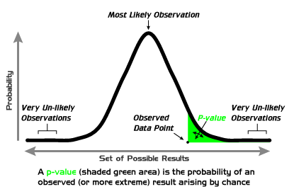
The p-value is calculated after you collect data. It tells you the probability of getting a sample result as extreme as (or more extreme than) what you observed, assuming the null hypothesis is true.

The decision rule is straightforward:

• Reject $H_0$ if p-value < $\alpha$
• Fail to reject $H_0$ if p-value ≥ $\alpha$

For example, if you set $\alpha = 0.05$ and your test produces a p-value of 0.02, you reject $H_0$ because 0.02 < 0.05. The sample data is unlikely enough under $H_0$ that you have evidence against it.

One thing that trips people up: "fail to reject" is not the same as "accept." You're never proving $H_0$ is true. You're just saying you didn't find enough evidence against it.

The rejection region is the set of test statistic values that would lead you to reject $H_0$. It corresponds directly to your chosen $\alpha$.

Types of hypothesis tests

The direction of your alternative hypothesis ($H_a$) determines what kind of test you run.

• Left-tailed test: $H_a$ claims the parameter is less than a specific value
  • The critical region sits in the left tail of the distribution
  • Example: $H_a: \mu < 100$
• Right-tailed test: $H_a$ claims the parameter is greater than a specific value
  • The critical region sits in the right tail
  • Example: $H_a: p > 0.5$
• Two-tailed test: $H_a$ claims the parameter is not equal to a specific value
  • The critical region is split between both tails, with $\alpha/2$ in each
  • Example: $H_a: \mu \neq 75$

How do you choose? Think about the research question. If you only care whether something is lower (or only whether it's higher), use a one-tailed test. If you care about any difference in either direction, use two-tailed.

Hypothesis testing for proportions

When you're testing a claim about a population proportion, you use a z-test. Here's the full process:

1. State the hypotheses.

   • Null hypothesis: $H_0: p = p_0$ (the population proportion equals some claimed value)
   • Alternative hypothesis: $H_a: p < p_0$, $H_a: p > p_0$, or $H_a: p \neq p_0$, depending on the research question

2. Set the significance level ($\alpha$) and identify the test type (left-tailed, right-tailed, or two-tailed).

3. Calculate the test statistic using the formula:

$z = \frac{\hat{p} - p_0}{\sqrt{\frac{p_0(1 - p_0)}{n}}}$

• $\hat{p}$ = sample proportion (successes divided by sample size)
• $p_0$ = the proportion claimed in $H_0$
• $n$ = sample size
• The denominator is the standard error, which measures how much $\hat{p}$ typically varies from $p_0$ due to random sampling

1. Find the p-value using the z-score and the standard normal distribution:

   • Left-tailed: p-value = $P(Z < z)$
   • Right-tailed: p-value = $P(Z > z)$
   • Two-tailed: p-value = $2 \cdot P(Z > |z|)$

2. Make a decision.

   • Reject $H_0$ if p-value < $\alpha$
   • Fail to reject $H_0$ if p-value ≥ $\alpha$

3. Interpret the result in context. Don't just say "reject" or "fail to reject." Translate the conclusion back into the language of the problem.

Worked example: A company claims that 60% of customers prefer their product. You survey 200 people and find that 108 prefer it ($\hat{p} = 0.54$). Test at $\alpha = 0.05$ whether the true proportion is less than 0.60.

• $H_0: p = 0.60$, $H_a: p < 0.60$ (left-tailed)
• $z = \frac{0.54 - 0.60}{\sqrt{\frac{0.60(0.40)}{200}}} = \frac{-0.06}{\sqrt{0.0012}} = \frac{-0.06}{0.03464} \approx -1.73$
• p-value = $P(Z < -1.73) \approx 0.0418$
• Since 0.0418 < 0.05, reject $H_0$
• Conclusion: There is sufficient evidence at the 0.05 level to suggest that the true proportion of customers who prefer the product is less than 60%.

Additional Considerations in Hypothesis Testing

A few more concepts that come up alongside hypothesis testing:

• Confidence interval: A range of plausible values for the population parameter. If a 95% confidence interval for $p$ doesn't contain $p_0$, that's consistent with rejecting $H_0$ at $\alpha = 0.05$. Confidence intervals and hypothesis tests are closely related.
• Statistical power: The probability of correctly rejecting $H_0$ when it's actually false (i.e., detecting a real effect). Power increases with larger sample sizes and larger effect sizes. Low power means you might miss a real difference.
• Effect size: Measures how big the difference is, not just whether it exists. A statistically significant result can have a tiny effect size, which may not matter in practice.
• Degrees of freedom: The number of independent values in a dataset that are free to vary. This concept matters more when you move to t-tests (coming up soon), where degrees of freedom affect the shape of the distribution you use.