5.1 Continuous Probability Functions

Continuous Probability Distributions

Area under probability density curves

A probability density function (PDF), written as $f(x)$, describes how probability is spread across the possible values of a continuous random variable $x$. Unlike discrete distributions where you can ask "what's the probability of exactly 5?", the probability of any single exact value in a continuous distribution is always zero. This sounds strange at first, but it makes sense: there are infinitely many possible values, so probability only has meaning over an interval.

To find the probability that a continuous random variable falls within a range, you calculate the area under the PDF curve between two limits:

$P(a \leq X \leq b) = \int_{a}^{b} f(x) dx$

where $a$ is the lower limit, $b$ is the upper limit, and $\int$ represents the integral (which gives you the area under the curve).

In practice, you can find this area using:

• Integration techniques like the Fundamental Theorem of Calculus
• Technology such as graphing calculators or statistical software (which is what you'll use most of the time in an intro course)

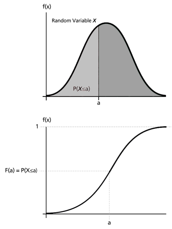
The cumulative distribution function (CDF) is a related tool. It gives the probability that the random variable takes a value less than or equal to a given point. So $F(x) = P(X \leq x)$. If you need $P(X \leq 3)$, that's just the CDF evaluated at 3.

Probability-area relationship in distributions

In continuous distributions, probability and area are the same thing. A larger area under the curve between two points means a higher probability of the variable landing in that range.

The shape of the PDF tells you how probability is distributed:

• A normal distribution (bell-shaped curve) concentrates the highest probability around the mean, with lower probabilities in the tails. About 68% of the area falls within one standard deviation of the mean, while only about 0.3% falls beyond three standard deviations.
• A continuous uniform distribution has a flat, constant density over a finite interval. Every subinterval of the same width has equal probability. For example, if a random variable is uniformly distributed between 0 and 10, the probability of landing between 2 and 4 is the same as landing between 7 and 9.

The key takeaway: wherever the curve is taller, outcomes in that region are more likely. Wherever it's lower, outcomes are less likely.

Total area of density functions

The total area under any valid PDF curve is exactly 1:

$\int_{-\infty}^{\infty} f(x) dx = 1$

This is a fundamental requirement. Since the random variable must take some value, the probabilities across all possible outcomes need to sum to 1. If a function's total area doesn't equal 1, it's not a valid PDF.

This property is also a useful problem-solving tool. If you know the area under one portion of the curve, you can find the area under the remaining portion by subtracting from 1.

This "complement" approach often saves time, especially when it's easier to calculate the probability you don't want and subtract it from 1.

Additional Probability Concepts

• Probability axioms are the foundational rules of probability theory. The two most relevant here: every probability is between 0 and 1, and the total probability across all outcomes equals 1. These axioms are exactly why the total area under a PDF must be 1.
• Random variable transformations involve changing the scale or form of a random variable (for instance, taking the log or squaring it), which changes its distribution. You'll encounter this more in later units, but it's worth knowing that transforming a variable can turn one type of distribution into another.