11.1 Facts About the Chi-Square Distribution

Key Characteristics and Properties

The chi-square distribution is a probability distribution used to analyze categorical data. You'll rely on it for goodness-of-fit tests and for checking whether two categorical variables are related. It behaves differently from the normal distribution in some important ways, so understanding its shape and properties matters.

Shape and Behavior

The chi-square distribution is a continuous distribution defined by a single parameter: degrees of freedom ($df$), which must be a positive integer.

A few defining features:

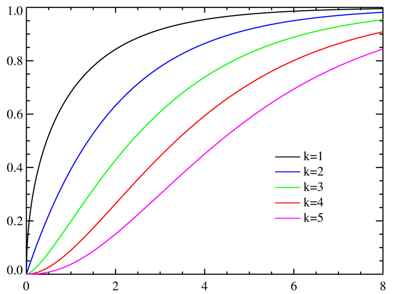
• It only takes non-negative values, ranging from 0 to positive infinity. You'll never get a negative chi-square value.
• It's right-skewed (positively skewed). The tail stretches out to the right.
• The skewness depends on $df$. When $df = 1$, the curve is heavily skewed. As $df$ increases, the peak shifts rightward and the curve becomes more symmetric, gradually approaching the shape of a normal distribution.

Think of it this way: a chi-square distribution with 3 degrees of freedom looks very lopsided, but one with 50 degrees of freedom looks close to a bell curve.

Mean, Variance, and Standard Deviation

These formulas are straightforward and worth memorizing:

• Mean: $\mu = df$
• Variance: $\sigma^2 = 2(df)$
• Standard deviation: $\sigma = \sqrt{2(df)}$

So for a chi-square distribution with $df = 10$, the mean is 10, the variance is 20, and the standard deviation is $\sqrt{20} \approx 4.47$.

Notice that the mean equals the degrees of freedom. That's a quick way to check your work: the center of the distribution should sit right at $df$.

Relationship to the Normal Distribution

The chi-square distribution is built from the normal distribution. If you take independent standard normal random variables $Z_1, Z_2, \ldots, Z_n$ and square each one, their sum follows a chi-square distribution:

$\sum_{i=1}^{n} Z_i^2 \sim \chi^2(n)$

This means a chi-square distribution with $n$ degrees of freedom is literally the sum of $n$ squared standard normal values.

A practical consequence: when $df$ is large (roughly $df > 30$), the chi-square distribution can be approximated by a normal distribution with $\mu = df$ and $\sigma = \sqrt{2(df)}$. This is why chi-square tables sometimes stop at moderate $df$ values; beyond that, you can use the normal approximation.

Applications in Statistical Inference

You'll encounter the chi-square distribution in two main types of tests in this course:

• Goodness-of-fit tests compare observed frequencies to expected frequencies. For example, you might test whether the distribution of colors in a bag of candy matches what the manufacturer claims.
• Tests of independence use contingency tables to assess whether two categorical variables are related. For instance, you could test whether preferred study method (flashcards, re-reading, practice problems) is independent of grade level.

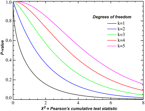
In both cases, you calculate a chi-square test statistic, then compare it to a critical value from the chi-square distribution to decide whether to reject the null hypothesis. Larger test statistic values fall further into the right tail, making rejection of the null hypothesis more likely.