12.1 Linear Equations

Linear Equations

Linear equations describe the relationship between two variables using a straight line. They're the building block for linear regression, which you'll use throughout statistics to model data, measure relationships, and make predictions.

This section covers the components of a linear equation (slope and y-intercept), how to interpret them in context, how to graph them, and how they connect to the line of best fit in regression.

Linear Equations

Construction of linear equations

The general form of a linear equation is:

$y = mx + b$

• $m$ is the slope of the line. It tells you how much $y$ changes when $x$ increases by one unit.
• $b$ is the y-intercept. It's the value of $y$ when $x = 0$, which is where the line crosses the y-axis.

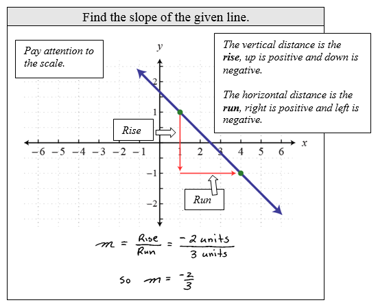
To find the slope between any two points, use the slope formula:

$m = \frac{y_2 - y_1}{x_2 - x_1}$

This is just "rise over run." You're dividing the vertical change by the horizontal change between two points on the line.

To construct a linear equation, you need to know both the slope and the y-intercept. For example, if a line has a slope of 2 and a y-intercept of -3, the equation is $y = 2x - 3$.

Interpretation of slope and y-intercept

In a statistics context, slope and y-intercept carry real-world meaning tied to whatever variables you're studying.

Slope ($m$) represents the predicted change in the dependent variable ($y$) for every one-unit increase in the independent variable ($x$). For example, if you're modeling the relationship between hours studied ($x$) and exam score ($y$), a slope of 5 means that each additional hour of studying is associated with a 5-point increase in exam score.

Y-intercept ($b$) represents the predicted value of $y$ when $x = 0$. Using the same example, a y-intercept of 40 would mean a student who studies zero hours is predicted to score 40 on the exam. Keep in mind that the y-intercept doesn't always make practical sense. If $x = 0$ falls outside the range of your data, treat the y-intercept as a mathematical starting point rather than a meaningful prediction.

The correlation coefficient (covered later in this unit) measures how strong the linear relationship is between the two variables.

Graphing of linear equations

Graphing a linear equation lets you visualize the relationship between $x$ and $y$. Here's how to do it:

1. Identify the slope ($m$) and y-intercept ($b$) from the equation.
2. Plot the y-intercept on the graph. This is the point $(0, b)$.
3. From the y-intercept, use the slope to find a second point. Move 1 unit to the right and $m$ units up (or down if $m$ is negative).
4. Plot the second point and draw a straight line through both points.

For example, with $y = 2x - 3$: plot $(0, -3)$, then move 1 right and 2 up to get $(1, -1)$. Connect those points with a line.

Key features to identify on a graph:

• x-intercept: where the line crosses the x-axis ($y = 0$). You can find this by setting $y = 0$ and solving for $x$.
• y-intercept: where the line crosses the y-axis ($x = 0$).
• Slope direction: a positive slope goes upward left to right, a negative slope goes downward, and a zero slope is a flat horizontal line.

When working with real data, a scatter plot displays the individual data points so you can see whether a linear model is a reasonable fit before drawing a line through them.

Linear Regression and Best Fit

Linear regression finds the single straight line that best summarizes the relationship in your data. The method used is called least squares, which minimizes the sum of the squared residuals.

A residual is the vertical distance between an actual data point and the value predicted by the line. In other words: $\text{residual} = \text{observed } y - \text{predicted } y$. Some residuals are positive (point above the line) and some are negative (point below the line). The least squares method finds the line where the total of all squared residuals is as small as possible.

Once you have a line of best fit, you can use it for:

• Interpolation: predicting $y$ for an $x$ value within the range of your observed data. These predictions tend to be more reliable.
• Extrapolation: predicting $y$ for an $x$ value outside the range of your data. These predictions are riskier because you're assuming the linear pattern continues beyond what you've actually observed.