9.6 Solving Systems with Gaussian Elimination

Matrices and Systems of Equations

Matrices give you a compact way to represent an entire system of linear equations, stripping away the variables so you can focus on the numbers. Once a system is in matrix form, you can apply systematic row operations to solve it. This section covers how to move between equation form and matrix form, and how row operations work.

more resources to help you study

practice questions

Augmented Matrices from Equations

An augmented matrix is a matrix that holds all the information from a system of equations: the coefficients on the left side and the constants on the right, separated by a vertical line.

To build an augmented matrix from a system:

1. Write each equation in standard form (all variables on the left in the same order, constants on the right).
2. Pull out the coefficients of each variable and the constant for each equation.
3. Place each equation's numbers in its own row. The constants go in the last column, separated by a vertical line.

For example, the system:

$2x + 3y - z = 7$

$x - y + 4z = -2$

$3x + 2y + z = 5$

becomes the augmented matrix:

$\left[\begin{array}{ccc|c} 2 & 3 & -1 & 7 \\ 1 & -1 & 4 & -2 \\ 3 & 2 & 1 & 5 \end{array}\right]$

If a variable is missing from an equation, use 0 as its coefficient.

Going the other direction is straightforward: each row becomes an equation. The first column corresponds to $x$, the second to $y$, and so on, with the last column giving the constant after the equals sign.

Transformation Through Row Operations

You can transform an augmented matrix using three elementary row operations, none of which change the solution set:

• Row interchange: Swap two rows. Notation: $R_i \leftrightarrow R_j$
• Row scaling: Multiply every entry in a row by a nonzero constant. Notation: $kR_i \rightarrow R_i$
• Row replacement (row addition): Add a multiple of one row to another row. Notation: $R_i + kR_j \rightarrow R_i$

The goal of these operations is to create zeros in strategic positions, transforming the matrix into row echelon form (upper triangular shape with leading 1s) or reduced row echelon form (leading 1s with zeros both above and below each pivot).

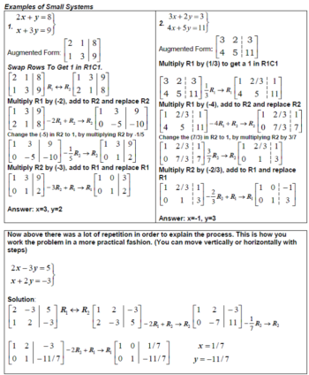
Gaussian Elimination

Gaussian Elimination for Linear Systems

Gaussian elimination is a step-by-step process that uses row operations to solve a system. Here's how it works:

Phase 1: Forward elimination (get to row echelon form)

1. Start with the leftmost column that has a nonzero entry. This is your first pivot column.
2. If needed, swap rows so the pivot position has a nonzero entry (preferably 1).
3. Use row replacement to create zeros in every entry below the pivot.
4. Move to the next column and the next row down. Repeat steps 2–3 until the matrix has an upper triangular shape.

Phase 2: Back-substitution

1. Start with the bottom row (which should have the fewest unknowns) and solve for that variable.
2. Substitute that value into the equation above it and solve for the next variable.
3. Continue working upward until all variables are found.

Example: Suppose forward elimination gives you:

$\left[\begin{array}{ccc|c} 1 & 2 & -1 & 3 \\ 0 & 1 & 3 & -1 \\ 0 & 0 & 1 & 2 \end{array}\right]$

From the bottom row: $z = 2$. The second row gives $y + 3(2) = -1$, so $y = -7$. The first row gives $x + 2(-7) - 2 = 3$, so $x = 19$.

Gauss-Jordan elimination takes this further. Instead of back-substituting, you continue using row operations to create zeros above each pivot as well. The result is reduced row echelon form, where each pivot is 1 and every other entry in a pivot column is 0. You can read the solution directly from the matrix without any substitution.

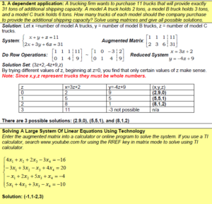
Interpretation of Matrix Solutions

Once your matrix is in row echelon or reduced row echelon form, the structure of the matrix tells you what kind of solution the system has:

• Unique solution: Every variable column contains a pivot. You can read off exactly one value for each variable.
• No solution (inconsistent): A row has all zeros for the coefficient entries but a nonzero constant, like $[0 \quad 0 \quad 0 \mid 5]$. This translates to $0 = 5$, which is impossible.
• Infinitely many solutions (dependent): There are fewer pivots than variables, meaning at least one variable is free (its column has no pivot). Assign a parameter (like $t$) to each free variable and express the pivot variables in terms of those parameters.

After finding a solution, always verify it by substituting back into the original equations. This catches arithmetic errors and confirms the solution makes sense in context.

Matrix and System Components

• Coefficients: The numbers multiplied by variables in each equation, which become the main entries of the matrix.
• Variables: The unknowns ($x, y, z$, etc.) represented by the columns of the coefficient portion of the matrix.
• Pivot: The leading nonzero entry in a row after the matrix is in echelon form. Pivots determine which variables are solved directly.
• Free variable: A variable whose column contains no pivot. These can take any value, leading to infinitely many solutions.
• Solution set: The collection of all ordered sets of values that satisfy every equation in the system simultaneously.