9.5 Matrices and Matrix Operations

Matrix Operations and Applications

Matrices give you a structured way to organize numbers into rows and columns, then perform operations on them as a single object. In this unit, they become your primary tool for representing and solving systems of linear equations, which connects everything you've learned about systems into a compact, powerful framework.

more resources to help you study

practice questions

Matrix arithmetic operations

Addition and subtraction only work when both matrices have the same dimensions. You add (or subtract) the corresponding entries, position by position. A $2 \times 3$ matrix can only be added to another $2 \times 3$ matrix, and the result is also $2 \times 3$.

For example:

$\begin{bmatrix} 1 & 4 \\ 2 & 5 \end{bmatrix} + \begin{bmatrix} 3 & 0 \\ -1 & 6 \end{bmatrix} = \begin{bmatrix} 4 & 4 \\ 1 & 11 \end{bmatrix}$

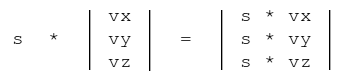
Scalar multiplication means multiplying every element in the matrix by a single constant:

$2 \begin{bmatrix} 1 & 2 \\ 3 & 4 \end{bmatrix} = \begin{bmatrix} 2 & 4 \\ 6 & 8 \end{bmatrix}$

The result keeps the same dimensions as the original.

Properties to know:

• Commutative property of addition: $A + B = B + A$
• Associative property of addition: $(A + B) + C = A + (B + C)$
• Distributive property of scalar multiplication over addition: $k(A + B) = kA + kB$
• Associative property of scalar multiplication: $(kl)A = k(lA)$

These behave just like the properties you already know from regular algebra, which makes them straightforward to apply.

Conditions for matrix multiplication

Matrix multiplication is where things get more involved. Two matrices can only be multiplied if the number of columns in the first matrix equals the number of rows in the second. A $2 \times 3$ matrix can multiply a $3 \times 4$ matrix, and the result will be $2 \times 4$.

Think of it as: inner dimensions must match, outer dimensions give the result size.

To compute each entry of the product, follow this process:

1. Pick a row from the first matrix and a column from the second matrix.
2. Multiply corresponding elements together.
3. Add up all those products. That sum is one entry in the result.
4. Repeat for every row-column combination.

For example, if you're finding entry $c_{11}$ of the product $AB$:

$c_{11} = a_{11}b_{11} + a_{12}b_{21} + a_{13}b_{31}$

Properties of matrix multiplication:

• Not commutative: $AB \neq BA$ in general. This is a big difference from regular number multiplication. Even when both products are defined, they usually give different results.
• Associative: $(AB)C = A(BC)$
• Distributive over addition: $A(B + C) = AB + AC$ and $(A + B)C = AC + BC$

The identity matrix is the matrix equivalent of the number 1. It's a square matrix with 1s along the main diagonal and 0s everywhere else, denoted $I_n$ for an $n \times n$ matrix:

$I_2 = \begin{bmatrix} 1 & 0 \\ 0 & 1 \end{bmatrix}$

Multiplying any matrix $A$ by the identity (with compatible dimensions) returns $A$ unchanged: $AI_n = I_nA = A$.

Applications in linear systems

Matrices let you rewrite an entire system of equations as a single matrix equation. Take the system:

$2x + 3y = 5$ $4x - y = 3$

You can break this into three matrices:

• Coefficient matrix $A$: $\begin{bmatrix} 2 & 3 \\ 4 & -1 \end{bmatrix}$ (the numbers in front of the variables)
• Variable matrix $X$: $\begin{bmatrix} x \\ y \end{bmatrix}$
• Constant matrix $B$: $\begin{bmatrix} 5 \\ 3 \end{bmatrix}$ (the right-hand side values)

The system becomes $AX = B$. To solve:

1. Write the system as $AX = B$.
2. Find the inverse of the coefficient matrix, $A^{-1}$ (this only exists if $A$ is invertible).
3. Multiply both sides on the left by $A^{-1}$: $A^{-1}AX = A^{-1}B$.
4. Since $A^{-1}A = I$, this simplifies to $X = A^{-1}B$.

Existence and uniqueness of solutions:

• Unique solution: The coefficient matrix $A$ is invertible (its determinant is nonzero).
• Infinitely many solutions: The rank of the augmented matrix $[A|B]$ equals the rank of $A$, but both are less than the number of variables.
• No solution: The rank of $[A|B]$ is greater than the rank of $A$, meaning the equations contradict each other.

Advanced matrix concepts

These topics go beyond the core operations but show up in honors-level problems and connect to future coursework.

Determinant: A scalar value computed from a square matrix. For a $2 \times 2$ matrix $\begin{bmatrix} a & b \\ c & d \end{bmatrix}$, the determinant is $ad - bc$. If the determinant is zero, the matrix has no inverse and the corresponding system either has no solution or infinitely many.

Transpose: Flip a matrix over its main diagonal so that rows become columns and columns become rows. Denoted $A^T$. For example:

$\begin{bmatrix} 1 & 2 \\ 3 & 4 \\ 5 & 6 \end{bmatrix}^T = \begin{bmatrix} 1 & 3 & 5 \\ 2 & 4 & 6 \end{bmatrix}$

Eigenvalues and eigenvectors: For a square matrix $A$, an eigenvector $v$ is a nonzero vector that, when multiplied by $A$, only gets scaled (not rotated). The scaling factor is the eigenvalue $\lambda$, satisfying $Av = \lambda v$. You'll encounter these more in linear algebra, but they're worth knowing exist since they're central to analyzing transformations.