8.7 Parametric Equations: Graphs

Graphing Parametric Equations

Parametric equations describe curves by defining $x$ and $y$ separately as functions of a third variable, called a parameter (usually $t$). Instead of writing $y$ directly in terms of $x$, you let both coordinates depend on $t$. This is especially useful for modeling motion, where $t$ often represents time, and for describing curves that can't be written as a single function $y = f(x)$.

Plotting Parametric Curves

In parametric form, every point on a curve comes from a pair of equations:

• $x = x(t)$
• $y = y(t)$

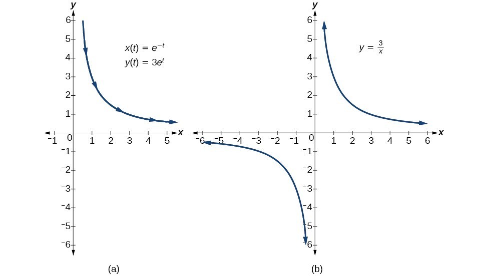
As $t$ changes, the point $(x(t), y(t))$ traces out a path on the Cartesian plane. The direction the curve is traced (as $t$ increases) is called the orientation.

To graph a parametric curve by hand:

1. Choose several values of $t$ across the given interval.
2. Plug each $t$ into both $x(t)$ and $y(t)$ to get coordinate pairs.
3. Plot the resulting $(x, y)$ points.
4. Connect the points with a smooth curve, using arrows to show the direction of increasing $t$.

For example, if $x(t) = t + 1$ and $y(t) = t^2$ for $-2 \leq t \leq 2$, you'd build a table:

Plotting these points and connecting them reveals a parabola opening upward, traced from left-to-right as $t$ increases.

Interpreting Common Parametric Graphs

Circles centered at the origin use the Pythagorean identity $\cos^2(t) + \sin^2(t) = 1$:

• $x(t) = r\cos(t)$, $y(t) = r\sin(t)$, where $r$ is the radius and $0 \leq t \leq 2\pi$

The curve traces counterclockwise starting from $(r, 0)$. If you want a circle centered at $(h, k)$ instead, shift the equations: $x(t) = h + r\cos(t)$, $y(t) = k + r\sin(t)$.

Ellipses centered at the origin work the same way but with different stretches along each axis:

• $x(t) = a\cos(t)$, $y(t) = b\sin(t)$, where $a$ is the semi-major axis length and $b$ is the semi-minor axis length (assuming $a > b$), with $0 \leq t \leq 2\pi$

Projectile motion is a classic application where $t$ literally represents time:

• $x(t) = v_0 \cos(\theta)\, t$
• $y(t) = v_0 \sin(\theta)\, t - \frac{1}{2}gt^2$

Here $v_0$ is the initial speed, $\theta$ is the launch angle above horizontal, and $g$ is gravitational acceleration ($9.8 \text{ m/s}^2$). The $x$-equation gives constant horizontal velocity, while the $y$-equation accounts for gravity pulling the object down. The resulting path is a parabola.

Lissajous figures result from combining two sinusoidal functions with different frequencies, such as $x(t) = \sin(at)$ and $y(t) = \sin(bt)$. Changing the ratio $a:b$ produces different looping patterns. These show up in physics when analyzing oscillations.

Conversion Between Parametric and Cartesian Forms

Parametric → Cartesian:

1. Solve one of the parametric equations for $t$.
2. Substitute that expression into the other equation.
3. Simplify to get a single equation in $x$ and $y$.

For trig-based parametric equations, a different strategy often works better: use a trig identity to eliminate $t$. For instance, given $x = r\cos(t)$ and $y = r\sin(t)$, square both equations and add them to get $x^2 + y^2 = r^2$.

Cartesian → Parametric:

1. Introduce a parameter $t$.
2. Express $x$ and $y$ each in terms of $t$ so that the original Cartesian equation is satisfied.

There's no single "right" answer here. For example, $y = x^2$ could become $x = t$, $y = t^2$, or equally $x = 2t$, $y = 4t^2$. Both are valid parametrizations of the same curve.

Advanced Parametric Concepts

These topics go beyond basic graphing but connect to ideas you'll see in calculus:

• Tangent lines to parametric curves use the relationship $\frac{dy}{dx} = \frac{dy/dt}{dx/dt}$, provided $dx/dt \neq 0$. This gives the slope at any point along the curve.
• Arc length of a parametric curve from $t = a$ to $t = b$ is calculated with $\int_a^b \sqrt{\left(\frac{dx}{dt}\right)^2 + \left(\frac{dy}{dt}\right)^2}\, dt$.
• Vector-valued functions write parametric equations compactly as $\vec{r}(t) = \langle x(t), y(t) \rangle$, which extends naturally to three dimensions.