3.4 Graphs of Polynomial Functions

Polynomial Function Graphs

Polynomial functions produce smooth, continuous curves whose shapes are entirely determined by their algebraic form. By analyzing a polynomial's degree, leading coefficient, zeros, and multiplicity, you can sketch an accurate graph without plotting dozens of points.

more resources to help you study

practice questions

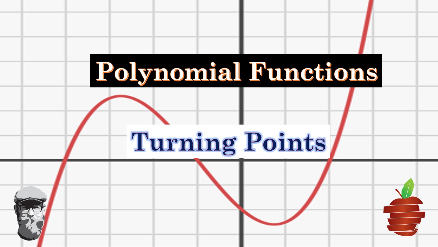
Features of Polynomial Function Graphs

Zeros (also called roots or x-intercepts) are the points where the graph crosses or touches the x-axis. These occur wherever $f(x) = 0$.

End behavior describes what happens to the graph as $x$ heads toward $+\infty$ or $-\infty$. Two things control it: the degree and the leading coefficient.

• Even degree polynomials have the same behavior on both ends (both arms go up, or both go down)
• Odd degree polynomials have opposite behavior on each end (one arm up, one arm down)
• A positive leading coefficient means the graph rises to the right; a negative leading coefficient means it falls to the right

Turning points (local maxima and minima) are where the graph changes from increasing to decreasing or vice versa. A polynomial of degree $n$ has at most $n - 1$ turning points.

Inflection points are where the graph changes concavity, shifting from curving upward to curving downward (or the reverse).

Factoring for Polynomial Zeros

To find the zeros of a polynomial:

1. Factor $f(x)$ completely. Use whatever technique fits: pull out common factors, factor by grouping, apply the difference of squares ($a^2 - b^2 = (a+b)(a-b)$), or use sum/difference of cubes.

2. Set each factor equal to zero and solve for $x$.

For example, if $f(x) = 2x^3 - 8x$, factor out $2x$ to get $2x(x^2 - 4) = 2x(x+2)(x-2)$. Setting each factor to zero gives zeros at $x = 0$, $x = -2$, and $x = 2$.

Degree and Graph Characteristics

The degree of a polynomial is the highest exponent on the variable. It tells you a lot about the graph:

• A polynomial of degree $n$ has at most $n$ zeros (counting both real and complex)
• It has at most $n - 1$ turning points
• The degree controls the end behavior (even vs. odd, as described above)
• Higher-degree polynomials can produce more complex shapes with more "wiggles"

Sketching Polynomial Function Graphs

1. Find the zeros by factoring or using the Rational Root Theorem and synthetic division.
2. Determine end behavior from the leading term. For instance, if the leading term is $-3x^5$, the degree is odd and the coefficient is negative, so the graph rises to the left and falls to the right.
3. Find the y-intercept by evaluating $f(0)$.
4. Identify turning points by analyzing where the function changes direction. In a pre-calculus context, you can estimate these by testing values between zeros or using a graphing calculator.
5. Plot the key points (zeros, y-intercept, turning points) and connect them with a smooth curve that matches the end behavior.

Advanced Polynomial Function Analysis

Intermediate Value Theorem for Roots

The Intermediate Value Theorem (IVT) says: if $f(x)$ is continuous on $[a, b]$ and $f(a)$ and $f(b)$ have opposite signs, then there's at least one value $c$ in $(a, b)$ where $f(c) = 0$.

Since all polynomials are continuous everywhere, the IVT always applies. This is useful when you can't factor easily. Evaluate $f(x)$ at a few integer values, and whenever the sign changes between two consecutive values, you know a root exists in that interval.

Multiplicity of Zeros and Graph Shape

Multiplicity is how many times a particular zero appears as a factor. For example, in $f(x) = (x - 3)^2(x + 1)$, the zero $x = 3$ has multiplicity 2 and $x = -1$ has multiplicity 1.

Multiplicity determines how the graph behaves at each zero:

• Odd multiplicity (1, 3, 5, ...): the graph crosses the x-axis at that zero
• Even multiplicity (2, 4, 6, ...): the graph touches the x-axis and bounces back without crossing

Higher multiplicity also makes the graph flatter near the zero. A zero with multiplicity 1 crosses sharply, while a zero with multiplicity 3 crosses with a flattened, S-shaped curve.

Polynomial Behavior from Algebraic Form

You can predict a lot about a polynomial's graph just from its equation:

• The leading term (degree and coefficient) determines end behavior
• The factored form reveals zeros and their multiplicities
• Complex zeros always come in conjugate pairs (like $2 + 3i$ and $2 - 3i$). They don't produce x-intercepts, but they do "use up" zeros from the total count. A degree-5 polynomial with 2 complex zeros will have only 3 real x-intercepts.

Continuity and Related Functions

Polynomial functions are continuous everywhere. There are no holes, jumps, or breaks in their graphs. This is what makes them predictable and smooth.

Rational functions (ratios of two polynomials) are a different story. They can have discontinuities wherever the denominator equals zero, which may produce vertical asymptotes or holes. Rational functions can also have horizontal or oblique asymptotes that describe end behavior. These concepts build directly on your understanding of polynomial graphs, and you'll explore them in the next sections of this unit.