The rectangular coordinate system is the foundation for visualizing algebraic relationships. It lets you plot points, represent equations, and analyze geometric shapes using a grid-like structure. This system is how numbers and equations connect to visual representations.
By mastering the coordinate plane, you can solve equations, create tables of values, and explore linear relationships. This knowledge forms the basis for more advanced topics in algebra and geometry.
Rectangular Coordinate System
Plot points on a rectangular coordinate plane
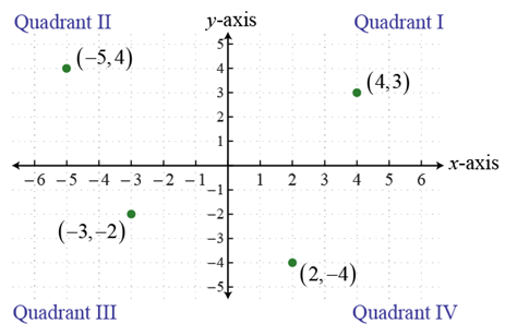
The rectangular coordinate plane (also called the Cartesian coordinate system) is built from two perpendicular number lines called axes:
- The x-axis runs horizontally (left to right)
- The y-axis runs vertically (bottom to top)
The point where the axes cross is called the origin, and its coordinates are (0, 0).
Every location on the plane is described by an ordered pair written as (x, y):
- The x-coordinate tells you how far to move left or right from the origin (positive = right, negative = left)
- The y-coordinate tells you how far to move up or down (positive = up, negative = down)
To plot a point, always start at the origin:
- Move along the x-axis by the amount of the x-coordinate
- From that spot, move parallel to the y-axis by the amount of the y-coordinate
- Mark the point
For example, to plot (3, 2), move 3 units right, then 2 units up. To plot (-1, -4), move 1 unit left, then 4 units down.

Solutions for two-variable equations
An ordered pair (x, y) is a solution to a two-variable equation if substituting those values into the equation makes it true.
To verify whether an ordered pair is a solution:
- Replace x with the first value and y with the second value
- Simplify both sides of the equation
- If the two sides are equal, the ordered pair is a solution; if not, it isn't
For the equation :
- (3, 2) is a solution because ✓
- (1, 1) is not a solution because ✗
Tables for linear equations
A linear equation in two variables has the form , where , , and are constants and and are not both zero. To find several solutions at once, you can build a table of values:
- Choose several values for one variable (x is the usual choice)
- Substitute each value into the equation and solve for the other variable
- Record each (x, y) pair in a table
For :
| x | y | Ordered Pair |
|---|---|---|
| 0 | 6 | (0, 6) |
| 1 | 4 | (1, 4) |
| 2 | 2 | (2, 2) |
| 3 | 0 | (3, 0) |
Each of these ordered pairs is a solution to the equation. You can verify any row by substituting back in: ✓
Solutions to linear equations
You can identify solutions to a linear equation in two ways: algebraically and graphically.
Algebraically: Substitute the x and y values from an ordered pair into the equation and check whether both sides are equal.
- (2, 3) is a solution to because ✓
- (1, 2) is not a solution to because ✗
Graphically: If you have the graph of a linear equation, any point that lies on the line is a solution. Any point off the line is not a solution. This is why graphing is so useful: the line itself is a picture of every possible solution.
Coordinate Geometry
Coordinate geometry combines algebra and geometry by placing geometric shapes on the coordinate plane. Once a shape is on the plane, you can use coordinates and equations to calculate distances, find midpoints, and describe lines or curves with algebraic formulas. This connection between algebra and geometry comes up repeatedly in later math courses.