7.3 Using the Central Limit Theorem

Central Limit Theorem

more resources to help you study

practice questions

Calculating Probabilities with the Central Limit Theorem

The Central Limit Theorem (CLT) tells you that the sampling distribution of the sample mean will be approximately normal as long as the sample size is large enough, typically $n \geq 30$. This holds regardless of the shape of the original population, whether it's skewed, uniform, or anything else. If the population itself is already normal, the sampling distribution of the mean is normal for any sample size, even something as small as $n = 5$.

This matters because once you know the sampling distribution is approximately normal, you can use the Z-distribution to calculate probabilities about sample means.

To find probabilities for a sample mean, follow these steps:

1. Identify the population mean $\mu$ and population standard deviation $\sigma$.

2. Calculate the mean of the sampling distribution: $\mu_{\bar{x}} = \mu$ (it equals the population mean).

3. Calculate the standard error (the standard deviation of the sampling distribution): $\sigma_{\bar{x}} = \frac{\sigma}{\sqrt{n}}$

4. Convert the sample mean to a Z-score: $Z = \frac{\bar{x} - \mu_{\bar{x}}}{\sigma_{\bar{x}}}$

5. Use a Z-table or calculator to find the probability.

Example: Suppose the population mean is 100, the population standard deviation is 20, and you draw samples of size 36. Then $\mu_{\bar{x}} = 100$ and $\sigma_{\bar{x}} = \frac{20}{\sqrt{36}} = 3.33$. If you want the probability that a sample mean exceeds 105, you'd compute $Z = \frac{105 - 100}{3.33} = 1.50$ and look up that Z-score.

Applying the CLT to sums of random variables:

The CLT also works for the sum of independent random variables, not just the mean. The formulas shift slightly:

• Mean of the sum: $\mu_{\Sigma x} = n\mu$
• Standard deviation of the sum: $\sigma_{\Sigma x} = \sqrt{n} \cdot \sigma$

For example, if you add 10 independent random variables each with mean 5 and standard deviation 2, then $\mu_{\Sigma x} = 10 \times 5 = 50$ and $\sigma_{\Sigma x} = \sqrt{10} \times 2 \approx 6.32$. You can then use the Z-distribution on the sum the same way you would for the mean.

Sample Size Effects on Distributions

Sample size controls two things about the sampling distribution: its shape and its spread.

Spread decreases as $n$ increases. The standard error formula $\sigma_{\bar{x}} = \frac{\sigma}{\sqrt{n}}$ means larger samples produce narrower sampling distributions. A narrower distribution means your sample mean is more likely to land close to the true population mean, giving you more precise estimates.

• If $\sigma = 10$ and $n = 25$: $\sigma_{\bar{x}} = \frac{10}{\sqrt{25}} = 2$
• If $\sigma = 10$ and $n = 100$: $\sigma_{\bar{x}} = \frac{10}{\sqrt{100}} = 1$

Quadrupling the sample size cuts the standard error in half. That's the $\sqrt{n}$ in the denominator at work.

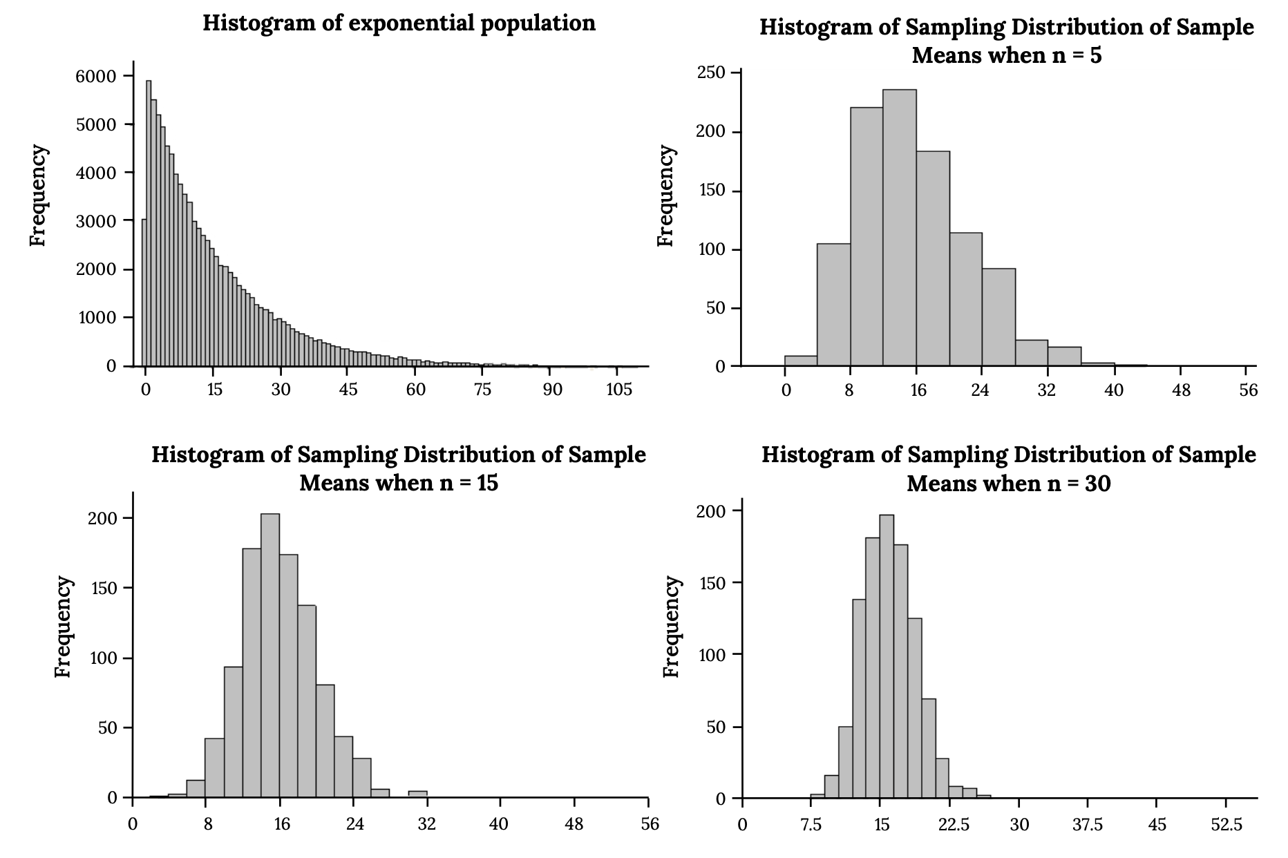
Shape becomes more normal as $n$ increases. For small samples drawn from non-normal populations (say, right-skewed income data with $n = 10$), the sampling distribution of the mean will still carry some of that skew. As you increase $n$, the distribution gradually becomes more symmetric and bell-shaped. By around $n = 30$, the normal approximation is typically reliable for most population shapes. Heavily skewed populations may need even larger samples.

Central Limit Theorem vs. Law of Large Numbers

These two theorems are related but say different things.

The Law of Large Numbers (LLN) says that as your sample size grows, the sample mean converges to the population mean. In other words, bigger samples give you more accurate point estimates. If you flip a fair coin 10 times, you might get 70% heads. Flip it 10,000 times, and you'll be very close to 50%.

The Central Limit Theorem goes further. It doesn't just say the sample mean gets closer to $\mu$; it tells you the shape of the sampling distribution. Specifically, the distribution of sample means becomes approximately normal for large $n$, which lets you calculate probabilities and build confidence intervals.

Think of it this way:

• LLN tells you where the sample mean will land (near $\mu$).
• CLT tells you the distribution of sample means around $\mu$ (approximately normal with standard error $\frac{\sigma}{\sqrt{n}}$).

Both are foundational for inferential statistics. The LLN justifies using sample means as estimates, and the CLT gives you the tools to quantify how confident you should be in those estimates.

Population Parameters and Sample Statistics

Population parameters describe the entire population. You usually don't know their exact values. Common ones include the population mean $\mu$ and population standard deviation $\sigma$.

Sample statistics are calculated from your data and serve as estimates of those parameters. The sample mean $\bar{x}$ estimates $\mu$, and the sample standard deviation $s$ estimates $\sigma$.

The CLT connects these two worlds. It describes how sample means are distributed around the population mean, which is what makes inferential statistics possible. When you run a hypothesis test, you're asking: "Given what the CLT tells me about the sampling distribution, is this sample mean surprising enough to reject my assumption about $\mu$?" When you build a confidence interval, you're using the CLT's normal approximation to create a range of plausible values for $\mu$.

This is why the CLT sits at the center of so many statistical methods. Without it, you'd have no principled way to go from sample data to conclusions about the population.