5.4 Continuous Distribution

Continuous Distributions

Continuous distributions model random variables that can take any value within a range, like heights, weights, or waiting times. Unlike discrete distributions where you sum probabilities for individual outcomes, continuous distributions use areas under curves (integrals) to find probabilities. This section covers the two main continuous distributions you need to know (uniform and exponential), how to read and interpret density functions, and how to calculate means and variances for continuous random variables.

Continuous Distributions

Continuous Probability Calculations

Continuous Uniform Distribution

A uniform distribution applies when every value in a range is equally likely. The PDF is flat, meaning no value is more probable than any other.

• PDF: $f(x) = \frac{1}{b-a}$ for $a \leq x \leq b$
• CDF: $F(x) = \frac{x-a}{b-a}$ for $a \leq x \leq b$
• Probability over an interval: $P(c \leq X \leq d) = \frac{d-c}{b-a}$ for $a \leq c \leq d \leq b$

Because the PDF is constant, probability calculations reduce to a simple ratio: the length of the interval you care about divided by the total length of the distribution's range. For example, if a random number is chosen uniformly between 0 and 1, the probability it falls between 0.2 and 0.5 is $\frac{0.5 - 0.2}{1 - 0} = 0.3$.

Exponential Distribution

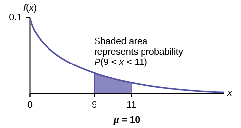
The exponential distribution models the time between events in a Poisson process, where events occur continuously and independently at a constant average rate $\lambda$.

• PDF: $f(x) = \lambda e^{-\lambda x}$ for $x \geq 0$
• CDF: $F(x) = 1 - e^{-\lambda x}$ for $x \geq 0$
• Survival probability (event hasn't occurred by time $x$): $P(X > x) = e^{-\lambda x}$

The memoryless property is unique to the exponential distribution among continuous distributions. It states:

$P(X > s + t \mid X > s) = P(X > t) \text{ for } s, t \geq 0$

This means the probability of waiting an additional $t$ units doesn't depend on how long you've already waited. For instance, if a light bulb's lifespan is exponentially distributed, a bulb that's been running for 1,000 hours is no more likely to fail in the next hour than a brand-new bulb.

Interpretation of Density Functions

Probability Density Function (PDF)

A PDF $f(x)$ describes the relative likelihood of a continuous random variable taking on a given value. Two critical rules govern every PDF:

• $f(x) \geq 0$ for all $x$ (the function is never negative)
• The total area under the curve equals 1

The value of $f(x)$ at a single point is not a probability. Instead, the area under $f(x)$ over an interval gives you the probability that $X$ falls in that interval. So $P(160 \leq X \leq 180)$ for a height distribution equals the area under the PDF curve between 160 cm and 180 cm.

This also means $P(X = c) = 0$ for any single value $c$. There's no area under a curve at a single point, so the probability of hitting any exact value is zero.

Cumulative Distribution Function (CDF)

The CDF $F(x)$ gives the probability that $X$ is less than or equal to $x$:

$F(x) = P(X \leq x) = \int_{-\infty}^{x} f(t) \, dt$

The CDF is the running total of area under the PDF from the left. Its key properties:

• Non-decreasing: as $x$ increases, $F(x)$ can only stay the same or go up
• Bounded: $\lim_{x \to -\infty} F(x) = 0$ and $\lim_{x \to \infty} F(x) = 1$
• Right-continuous: no jumps (for continuous distributions)

The quantile function is the inverse of the CDF. Given a probability $p$, the quantile function returns the value $x$ such that $F(x) = p$. This is how you find percentiles: the 90th percentile is the value where $F(x) = 0.90$.

To find the probability that $X$ falls between two values using the CDF:

$P(a \leq X \leq b) = F(b) - F(a)$

Analysis of Continuous Distributions

Expected Value (Mean)

The expected value is the "balance point" of the distribution, calculated as a weighted average across all possible values:

$E(X) = \int_{-\infty}^{\infty} x \, f(x) \, dx$

For the specific distributions covered here:

• Uniform on $[a, b]$: $E(X) = \frac{a + b}{2}$
• Exponential with rate $\lambda$: $E(X) = \frac{1}{\lambda}$

Linearity of expectation holds for continuous variables just as it does for discrete ones:

$E(aX + b) = aE(X) + b$

Variance and Standard Deviation

Variance measures how spread out the distribution is around the mean $\mu = E(X)$:

$Var(X) = \int_{-\infty}^{\infty} (x - \mu)^2 f(x) \, dx$

The computational formula is often easier to work with:

$Var(X) = E(X^2) - [E(X)]^2$

To use this, you calculate $E(X^2) = \int_{-\infty}^{\infty} x^2 f(x) \, dx$ separately, then subtract the square of the mean.

For the specific distributions:

• Uniform on $[a, b]$: $Var(X) = \frac{(b - a)^2}{12}$
• Exponential with rate $\lambda$: $Var(X) = \frac{1}{\lambda^2}$

Variance scales quadratically under linear transformations:

$Var(aX + b) = a^2 \, Var(X)$

Note that adding a constant $b$ shifts the distribution but doesn't change its spread, which is why $b$ drops out.

Standard deviation is the square root of variance: $\sigma = \sqrt{Var(X)}$. It's in the same units as $X$, making it more interpretable than variance.

Advanced Concepts in Continuous Distributions

• The normal distribution (Gaussian distribution) is a symmetric, bell-shaped distribution fully characterized by its mean $\mu$ and standard deviation $\sigma$. It shows up constantly in statistics because of the Central Limit Theorem.
• A moment-generating function $M_X(t) = E(e^{tX})$ provides a compact way to compute moments (mean, variance, etc.) and can uniquely identify a distribution.
• Kurtosis measures how heavy or light the tails of a distribution are compared to a normal distribution. High kurtosis means more extreme outliers are likely.
• The likelihood function is used in parameter estimation. Given observed data, it measures how probable those observations are for different parameter values, forming the basis of maximum likelihood estimation.

Applying Continuous Distributions

Continuous Probability Calculations

Uniform Distribution Applications

A bus arrives at a stop at a uniformly random time between 7:00 AM and 7:15 AM. What's the probability it arrives within the first 5 minutes?

1. Identify the parameters: $a = 0$, $b = 15$ (minutes after 7:00)
2. Apply the formula: $P(0 \leq X \leq 5) = \frac{5 - 0}{15 - 0} = \frac{1}{3} \approx 0.333$

A bolt's length is uniformly distributed between 9.9 cm and 10.1 cm. The probability its length falls between 9.95 cm and 10.05 cm is $\frac{10.05 - 9.95}{10.1 - 9.9} = \frac{0.10}{0.20} = 0.5$.

Exponential Distribution Applications

Customers arrive at a store at an average rate of 6 per hour, so $\lambda = 6$ per hour (or equivalently, $\lambda = 0.1$ per minute). The probability the next customer arrives within 10 minutes:

1. Use the CDF: $P(X \leq 10) = 1 - e^{-0.1 \times 10} = 1 - e^{-1} \approx 0.632$

The probability of waiting more than 10 minutes: $P(X > 10) = e^{-1} \approx 0.368$.

Interpretation of Density Functions

Reading a PDF

When you look at a PDF, pay attention to:

• Domain: the range of possible values (where $f(x) > 0$)
• Peaks (modes): where the distribution is most concentrated. A distribution can be unimodal (one peak), bimodal (two peaks), or multimodal.
• Symmetry and skewness: a symmetric PDF is a mirror image around its mean. If the right tail stretches further, it's right-skewed; if the left tail stretches further, it's left-skewed.

Remember that the height of the PDF at a point doesn't give you a probability directly. A PDF can even have values greater than 1 (for example, the uniform distribution on $[0, 0.5]$ has $f(x) = 2$). What matters is the area under the curve.

Using the CDF in Practice

The CDF converts questions about ranges into simple subtraction:

• $P(X \leq 5)$: read $F(5)$ directly
• $P(X > 5) = 1 - F(5)$
• $P(3 \leq X \leq 5) = F(5) - F(3)$

To find a percentile, you go in reverse: set $F(x) = p$ and solve for $x$.

Analysis of Continuous Distributions

Calculating Mean and Variance

For distributions beyond uniform and exponential, you'll need to integrate directly. The steps:

1. Verify the function is a valid PDF (non-negative and integrates to 1)
2. Compute $E(X) = \int x \, f(x) \, dx$ over the support
3. Compute $E(X^2) = \int x^2 \, f(x) \, dx$ over the support
4. Find variance using $Var(X) = E(X^2) - [E(X)]^2$

Comparing Distributions

The mean and variance together tell you a lot about how two distributions differ. For example, if two queuing systems both have exponential service times but different rates ($\lambda_1 = 2$ vs. $\lambda_2 = 5$ customers per minute), the second system has a shorter average wait ($\frac{1}{5} = 0.2$ min vs. $\frac{1}{2} = 0.5$ min) and less variability ($Var = \frac{1}{25}$ vs. $\frac{1}{4}$).

Changing distribution parameters affects both the center and spread. In the exponential case, increasing $\lambda$ decreases both the mean and the variance simultaneously, since both depend on $\lambda$.