10.1 Two Population Means with Unknown Standard Deviations

Comparing Two Population Means with Unknown Standard Deviations

When you want to compare the averages of two groups but don't know the population standard deviations (which is almost always the case with real data), you use a two-sample t-test. This test determines whether the difference between two sample means is statistically significant or just due to random sampling variability.

The core idea: calculate a t-statistic from your data, find the corresponding p-value, and compare it to your significance level to make a decision. This section covers the formula, degrees of freedom, effect size, and the errors you can make along the way.

more resources to help you study

practice questions

T-Statistic Calculation for Two Population Means

Before you can use this test, two assumptions need to hold:

• Both populations are approximately normally distributed (or sample sizes are large enough for the Central Limit Theorem to kick in)
• The two samples are independent, meaning the data in one group doesn't influence or relate to the data in the other

The test statistic formula is:

$t = \frac{\bar{x}_1 - \bar{x}_2}{\sqrt{\frac{s_1^2}{n_1} + \frac{s_2^2}{n_2}}}$

where:

• $\bar{x}_1$ and $\bar{x}_2$ are the sample means
• $s_1^2$ and $s_2^2$ are the sample variances
• $n_1$ and $n_2$ are the sample sizes

The numerator captures how far apart the two sample means are. The denominator is the standard error of the difference, which accounts for how much variability exists within each group and how large the samples are. A bigger difference in means or less variability produces a larger t-value, which is stronger evidence against the null hypothesis.

Setting up the hypotheses:

• Null hypothesis ($H_0$): $\mu_1 = \mu_2$ (no difference between population means)
• Alternative hypothesis ($H_a$) takes one of three forms depending on your research question:
  • Two-tailed: $\mu_1 \neq \mu_2$
  • Left-tailed: $\mu_1 < \mu_2$
  • Right-tailed: $\mu_1 > \mu_2$

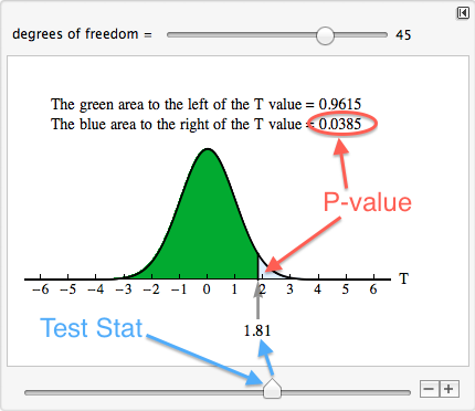
The p-value is the probability of observing a t-statistic at least as extreme as the one you calculated, assuming $H_0$ is true. If the p-value is less than your significance level ($\alpha$, typically 0.05), you reject $H_0$.

Quick example: Suppose Class A ($n_1 = 30$) scores an average of 78 with $s_1 = 10$, and Class B ($n_2 = 35$) scores an average of 83 with $s_2 = 12$. The numerator is $78 - 83 = -5$. The denominator is $\sqrt{\frac{100}{30} + \frac{144}{35}} = \sqrt{3.333 + 4.114} = \sqrt{7.447} \approx 2.729$. So $t \approx \frac{-5}{2.729} \approx -1.833$. You'd then compare this to the t-distribution with the appropriate degrees of freedom.

Degrees of Freedom in T-Distributions

Because the two samples can have different variances and different sizes, the degrees of freedom for this test aren't as simple as just adding sample sizes. You use the Welch-Satterthwaite equation:

$df = \frac{\left(\frac{s_1^2}{n_1} + \frac{s_2^2}{n_2}\right)^2}{\frac{\left(\frac{s_1^2}{n_1}\right)^2}{n_1-1} + \frac{\left(\frac{s_2^2}{n_2}\right)^2}{n_2-1}}$

This formula almost never gives a whole number, so you round down to the nearest integer. Rounding down is the conservative choice because it makes the critical value slightly larger, making it harder to reject $H_0$.

Why degrees of freedom matter:

• Smaller df produces a t-distribution with heavier tails, meaning you need a more extreme t-value to reach significance
• Larger df makes the t-distribution look more like the standard normal distribution
• Getting the df right ensures your p-value is accurate

For the example above, you'd plug the values into the Welch-Satterthwaite formula to get the exact df before looking up the p-value. In practice, your calculator or software handles this automatically.

Cohen's d for Effect Size

A statistically significant result doesn't necessarily mean the difference is practically meaningful. With a large enough sample, even a tiny difference can produce a small p-value. Cohen's d measures the actual size of the difference in standard deviation units.

$d = \frac{\bar{x}_1 - \bar{x}_2}{s_p}$

where $s_p$ is the pooled standard deviation:

$s_p = \sqrt{\frac{(n_1-1)s_1^2 + (n_2-1)s_2^2}{n_1 + n_2 - 2}}$

The pooled standard deviation is a weighted average of the two sample standard deviations, giving more weight to the larger sample.

Interpretation benchmarks (these are conventions, not rigid cutoffs):

• $d \approx 0.2$: small effect
• $d \approx 0.5$: medium effect
• $d \approx 0.8$: large effect

For instance, if two drugs lower blood pressure by an average difference of 3 mmHg with a pooled standard deviation of 6 mmHg, then $d = 3/6 = 0.5$, a medium effect. That tells you the difference is about half a standard deviation, which is clinically noticeable.

Cohen's d is independent of sample size, so you can compare effect sizes across different studies even when sample sizes vary widely.

Statistical Inference and Error Types

Every hypothesis test carries the risk of making the wrong conclusion. Understanding these errors helps you interpret results honestly.

• Type I error (false positive): You reject $H_0$ when it's actually true. The probability of this equals your significance level $\alpha$. If $\alpha = 0.05$, you accept a 5% chance of this error.
• Type II error (false negative): You fail to reject $H_0$ when it's actually false. The probability of this is denoted $\beta$.
• Statistical power = $1 - \beta$, the probability of correctly detecting a real difference. Power increases with larger sample sizes, larger effect sizes, and higher $\alpha$ levels.
• Confidence interval for the difference in means: Instead of just a yes/no decision, you can construct an interval estimate for $\mu_1 - \mu_2$. If the interval doesn't contain 0, that's consistent with rejecting $H_0$.

A common mistake: thinking "fail to reject $H_0$" means the two means are equal. It doesn't. It just means you didn't find enough evidence to conclude they're different, which could be because the sample was too small (low power) rather than because no difference exists.