3.6 Probability Topics

Probability Concepts

Probability gives you a precise way to measure how likely events are to occur. These tools show up everywhere in statistics, from hypothesis testing to modeling real-world risk in fields like finance and medicine. This section covers the core rules, counting techniques, and distributions you'll need.

more resources to help you study

practice questions

Rules of Probability Calculation

Every probability calculation builds on a few key rules. Choosing the right one depends on whether events are independent or dependent, and whether they're mutually exclusive or overlapping.

Addition Rule (OR problems)

Use this when you want the probability of at least one of two events happening.

• Mutually exclusive events (can't happen at the same time): $P(A \text{ or } B) = P(A) + P(B)$
  • Example: Flipping a coin once. Getting heads or tails are mutually exclusive, so $P(H \text{ or } T) = 0.5 + 0.5 = 1$.
• Non-mutually exclusive events (can overlap): $P(A \text{ or } B) = P(A) + P(B) - P(A \text{ and } B)$
  • Example: Drawing a heart or a face card from a standard deck. Some cards are both (jack, queen, king of hearts), so you subtract the overlap to avoid double-counting: $P = \frac{13}{52} + \frac{12}{52} - \frac{3}{52} = \frac{22}{52}$.

Multiplication Rule (AND problems)

Use this when you want the probability of two events both happening.

• Independent events (one doesn't affect the other): $P(A \text{ and } B) = P(A) \times P(B)$
  • Example: Rolling a 6 on a die twice in a row: $P = \frac{1}{6} \times \frac{1}{6} = \frac{1}{36}$.
• Dependent events (the first outcome changes the second): $P(A \text{ and } B) = P(A) \times P(B|A)$
  • Example: Drawing two aces from a deck without replacement. After drawing the first ace, only 3 aces remain among 51 cards: $P = \frac{4}{52} \times \frac{3}{51} = \frac{12}{2652} \approx 0.0045$.

Conditional Probability

$P(A|B) = \frac{P(A \text{ and } B)}{P(B)}$

This gives the probability of event A given that B has already occurred. The vertical bar $|$ means "given." For instance, the probability a patient actually has a disease given a positive test result is a conditional probability, and it's often surprisingly different from the test's raw accuracy.

Complement Rule

$P(A') = 1 - P(A)$

The probability of an event not happening equals 1 minus the probability it does happen. This is especially useful when calculating "at least one" problems, where it's easier to find the complement ("none") and subtract.

Counting Principles for Probabilities

Counting principles help you figure out the total number of possible outcomes, which you often need for the denominator of a probability fraction.

• Fundamental Counting Principle: If there are $n_1$ ways to do one thing and $n_2$ ways to do another, there are $n_1 \times n_2$ ways to do both. This extends to any number of stages. A restaurant with 4 main courses and 3 desserts offers $4 \times 3 = 12$ meal combinations.
• Permutations (order matters): The number of ways to arrange $r$ objects from a set of $n$:

$P(n, r) = \frac{n!}{(n-r)!}$

• Example: Arranging 3 books out of 7 on a shelf: $P(7,3) = \frac{7!}{4!} = 210$.
• Combinations (order doesn't matter): The number of ways to choose $r$ objects from $n$:

$C(n, r) = \binom{n}{r} = \frac{n!}{r!(n-r)!}$

• Example: Choosing 3 team members from a group of 7: $C(7,3) = \frac{7!}{3! \cdot 4!} = 35$. Notice this is smaller than the permutation count because different orderings of the same 3 people now count as one group.
• Permutations with repetition: When items can be reused, the count is $n^r$, where $n$ is the number of choices per position and $r$ is the number of positions. A 4-digit PIN using digits 0–9 has $10^4 = 10{,}000$ possibilities.
• Tree diagrams help visualize multi-step events. Each branch represents one outcome, and you multiply along branches to find the probability of a specific path.

Probability Distributions and Decisions

A probability distribution maps every possible value of a random variable to its probability. There are two main types:

• A discrete probability distribution applies when outcomes are countable (number of heads in 10 coin flips, number of customers per hour).
• A continuous probability distribution applies when outcomes can take any value in a range (heights, temperatures, time).

For discrete distributions, every probability must be between 0 and 1, and all probabilities must sum to exactly 1.

Expected Value

The expected value is the long-run average of a random variable. For a discrete random variable $X$:

$E(X) = \sum_{i=1}^{n} x_i \times P(X = x_i)$

You multiply each possible value by its probability, then add everything up. For example, if a game pays $10 with probability 0.3 and $0 with probability 0.7, the expected value is $10(0.3) + 0(0.7) = \$3$ per play.

Key properties of expected value:

1. Linearity: $E(aX + b) = aE(X) + b$ for constants $a$ and $b$
2. Addition: $E(X + Y) = E(X) + E(Y)$ (this holds whether or not $X$ and $Y$ are independent)

Note on property 2: the addition rule for expected value works for any two random variables. Independence is not required here, which is a common point of confusion.

Variance and Standard Deviation

Variance measures how spread out the distribution is around the mean:

$Var(X) = E[(X - \mu)^2] = E(X^2) - [E(X)]^2$

The second form (computational formula) is usually faster to calculate. Compute $E(X^2)$ by squaring each value, multiplying by its probability, and summing. Then subtract the square of the mean.

Standard deviation is the square root of variance:

$\sigma = \sqrt{Var(X)}$

Standard deviation is in the same units as the original variable, which makes it more interpretable than variance.

Law of Large Numbers

As the number of trials increases, the sample mean converges toward the expected value. This is why casinos are profitable in the long run even though individual gamblers sometimes win: over thousands of plays, the average outcome tracks the expected value closely.

Fundamental Concepts

These are the building blocks that everything above rests on.

• Sample space: The set of all possible outcomes in a probability experiment. For a single die roll, the sample space is $\{1, 2, 3, 4, 5, 6\}$. Defining it correctly is the first step in any probability problem.

• Probability axioms (the three rules all probabilities must follow):

  1. $0 \leq P(A) \leq 1$ for any event $A$
  2. $P(S) = 1$, where $S$ is the entire sample space
  3. For mutually exclusive events, $P(A \text{ or } B) = P(A) + P(B)$

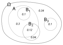
• Venn diagrams visually represent relationships between events. They're particularly helpful for seeing overlaps in non-mutually exclusive problems and for organizing information when applying the addition rule.