11.3 Test of Independence

Test of Independence

The chi-square test of independence determines whether two categorical variables are related or if they vary independently of each other. It compares what you actually observe in your data to what you'd expect to see if the two variables had no relationship at all.

more resources to help you study

practice questions

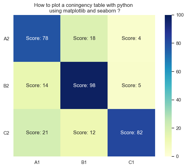
Construction of Contingency Tables

A contingency table (also called a two-way frequency table) organizes data for two categorical variables into rows and columns. Each cell shows the count of observations that fall into that particular combination of categories.

For example, suppose you survey 200 students about gender and preferred study method. Gender (male, female) forms the rows, and study method (alone, group, mixed) forms the columns. A cell might show that 45 females prefer studying in groups.

To build one:

1. Identify your two categorical variables.
2. List the categories (levels) for each variable along the rows and columns.
3. Count how many observations fall into each row-column combination and fill in the cells.
4. Add up each row and each column to get the marginal frequencies (the totals along the edges of the table).
5. Sum all observations to get the grand total.

The marginal frequencies matter because they're used directly in calculating expected values during the test.

Calculation of the Chi-Square Test Statistic

The test statistic follows a chi-square distribution, which is right-skewed and defined by degrees of freedom equal to $(r-1)(c-1)$, where $r$ is the number of rows and $c$ is the number of columns.

Step 1: Compute expected frequencies. For each cell, the expected frequency assumes the two variables are independent. The formula is:

$E_{ij} = \frac{(\text{row } i \text{ total}) \times (\text{column } j \text{ total})}{\text{grand total}}$

The logic here: if the variables are truly independent, the proportion in each cell should just reflect the product of its row and column proportions. You're asking, "If gender doesn't affect study preference at all, how many females should prefer group study based on the overall rates?"

Step 2: Calculate the test statistic.

$\chi^2 = \sum_{i=1}^{r} \sum_{j=1}^{c} \frac{(O_{ij} - E_{ij})^2}{E_{ij}}$

• $O_{ij}$ = observed frequency in row $i$, column $j$
• $E_{ij}$ = expected frequency in row $i$, column $j$

You compute $\frac{(O - E)^2}{E}$ for every single cell, then add them all up. Squaring the difference ensures that positive and negative deviations don't cancel out, and dividing by $E$ scales each contribution relative to how large the expected count is.

A larger $\chi^2$ value means the observed data deviates more from what independence would predict, which points toward a relationship between the variables.

Determination of Factor Independence

This is where you put it all together into a formal hypothesis test.

• Null hypothesis ($H_0$): The two categorical variables are independent (no association).
• Alternative hypothesis ($H_a$): The two categorical variables are dependent (there is an association).

Steps to conduct the test:

1. State $H_0$ and $H_a$.
2. Construct the contingency table and compute expected frequencies for every cell. (Check that all expected frequencies are at least 5; if not, the chi-square approximation may not be valid.)
3. Calculate the $\chi^2$ test statistic using the formula above.
4. Find degrees of freedom: $(r-1)(c-1)$. For a 2×3 table, that's $(2-1)(3-1) = 2$.
5. Choose a significance level (typically $\alpha = 0.05$).
6. Compare your test statistic to the critical value from the chi-square table, or find the p-value.

Making the decision:

• If $\chi^2 >$ critical value (or p-value $< \alpha$): reject $H_0$. You have evidence that the variables are associated. For instance, if your test statistic is 15.2 and the critical value at $df = 3$ and $\alpha = 0.05$ is 7.815, you reject $H_0$.
• If $\chi^2 <$ critical value (or p-value $> \alpha$): fail to reject $H_0$. There isn't sufficient evidence of a relationship. A test statistic of 3.5 compared to a critical value of 7.815 means you fail to reject.

Keep in mind that larger sample sizes give the test more power to detect real associations. A small sample might miss a genuine relationship simply because there isn't enough data.

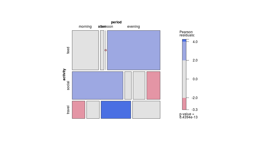
Additional Analysis

When you reject $H_0$, the test tells you the variables are associated, but it doesn't tell you where the association is strongest. Standardized residuals help with this. For each cell, the standardized residual is:

$\frac{O_{ij} - E_{ij}}{\sqrt{E_{ij}}}$

Cells with standardized residuals greater than about 2 or less than about $-2$ are the ones driving the significant result. This is useful for pinpointing which specific category combinations differ most from what independence would predict.