5.2 The Uniform Distribution

The uniform distribution models situations where every value within a set range is equally likely. It's one of the simplest continuous distributions you'll encounter, but it shows up often in probability problems involving waiting times, random number generation, and quality control.

Because the probability is spread evenly across the interval, calculating probabilities reduces to comparing lengths of intervals. That makes the formulas straightforward, but you still need to apply them carefully.

The Uniform Distribution

more resources to help you study

practice questions

Uniform Distribution Probability Calculations

A continuous uniform distribution assumes equal likelihood for all values within a specified interval. It's sometimes called a rectangular distribution because its probability density function forms a rectangle.

The notation is $X \sim U(a, b)$, where $a$ is the minimum value and $b$ is the maximum value.

Probability density function (PDF):

• $f(x) = \frac{1}{b - a}$ for $a \leq x \leq b$
• $f(x) = 0$ for $x < a$ or $x > b$

The height of the PDF, $\frac{1}{b-a}$, is just whatever constant makes the total area under the curve equal to 1. A wider interval means a shorter (lower) density, and a narrower interval means a taller density.

Cumulative distribution function (CDF):

• $F(x) = 0$ for $x < a$
• $F(x) = \frac{x - a}{b - a}$ for $a \leq x \leq b$
• $F(x) = 1$ for $x > b$

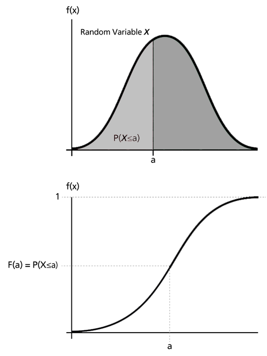
The CDF gives you $P(X \leq x)$, the probability that the outcome falls at or below a particular value. It climbs linearly from 0 to 1 across the interval.

Probability over a subinterval $[c, d]$ where $a \leq c \leq d \leq b$:

$P(c \leq X \leq d) = \frac{d - c}{b - a}$

This is just the length of the subinterval divided by the length of the full interval. You're finding what fraction of the total range your subinterval covers.

Equal Likelihood in Uniform Distributions

The defining feature of a uniform distribution is that all values in $[a, b]$ are equally probable. No part of the interval is "favored" over any other.

Two consequences follow from this:

• The probability of any single exact value is zero. Since $X$ is continuous, there are infinitely many possible values, so $P(X = c) = 0$ for any specific $c$. Probabilities only make sense over intervals.
• Probability is proportional to interval length. A subinterval twice as long has twice the probability. If you're asked about $P(7 \leq X \leq 9)$ versus $P(7 \leq X \leq 11)$ on the same uniform distribution, the second probability is exactly double the first because its subinterval is twice as wide.

Because $P(X = c) = 0$ for continuous distributions, it doesn't matter whether you write $P(c \leq X \leq d)$ or $P(c < X < d)$. The probability is the same either way. This is a detail that trips people up on exams, so keep it in mind.

Key Characteristics of Uniform Distributions

• Range: The interval $[a, b]$ defines all possible values.
• Mean: $\mu = \frac{a + b}{2}$, which is just the midpoint of the interval.
• Variance: $\sigma^2 = \frac{(b - a)^2}{12}$
• Standard deviation: $\sigma = \frac{b - a}{\sqrt{12}}$
• Constant density: The PDF is flat across the entire range, which is why the graph looks like a rectangle.
• Symmetry: The distribution is symmetric about its mean.

The mean and variance formulas are worth memorizing. The variance formula $\frac{(b-a)^2}{12}$ might look odd, but it comes from integrating $(x - \mu)^2$ across the uniform PDF. For an honors course, you should be comfortable deriving it if asked.

Applications of Uniform Distributions

When solving uniform distribution problems, follow these steps:

1. Identify $a$ and $b$ from the problem. These are the minimum and maximum values of the distribution.

2. Determine what probability you need. Are you looking for $P(X \leq d)$, $P(X \geq c)$, or $P(c \leq X \leq d)$?

3. Apply the correct formula.

   • For $P(X \leq d)$: use the CDF, $\frac{d - a}{b - a}$
   • For $P(X \geq c)$: use $1 - F(c) = \frac{b - c}{b - a}$
   • For $P(c \leq X \leq d)$: use $\frac{d - c}{b - a}$

4. Interpret the result in context. State what the probability means for the specific scenario.

Note on endpoints: for continuous uniform distributions, whether the interval is written as $[a, b]$ or $(a, b)$ doesn't affect probability calculations, since individual points have probability zero. This distinction matters for discrete distributions, but not here.