5.1 The chain rule for functions of several variables

The chain rule for functions of several variables extends the single-variable chain rule to composite functions where intermediate variables depend on one or more independent variables. Mastering this rule is essential for the rest of Calculus IV, since it underpins coordinate transformations, implicit differentiation in higher dimensions, and optimization with constrained variables.

Derivatives of Composite Functions

The Chain Rule and Composite Functions

In single-variable calculus, the chain rule says that if $y = f(g(t))$, then $\frac{dy}{dt} = f'(g(t)) \cdot g'(t)$. The multivariable chain rule does the same job, but now the "inner function" can output several variables, and the "outer function" can accept several inputs. Instead of multiplying two ordinary derivatives, you sum products of partial derivatives.

A composite function arises whenever one function feeds into another. For example, suppose $f(x, y) = x^2 + y^2$ and a path through the $xy$-plane is given by $x = t$, $y = t^3$. Then the composition $f(x(t), y(t)) = t^2 + t^6$ is a single-variable function of $t$ built from a two-variable function.

To set up the chain rule, identify two pieces:

• The outer function $f$, which takes the intermediate variables (here $x$ and $y$) as inputs.
• The inner functions (here $x(t)$ and $y(t)$), which express the intermediate variables in terms of the independent variable(s).

Partial Derivatives and the Total Derivative

Partial derivatives measure how $f$ changes when you vary one intermediate variable while freezing the others. For $f(x, y)$:

• $\frac{\partial f}{\partial x}$ is the rate of change of $f$ with respect to $x$, holding $y$ constant.
• $\frac{\partial f}{\partial y}$ is the rate of change of $f$ with respect to $y$, holding $x$ constant.

The total differential combines these into a single expression that captures how $f$ changes when all variables move at once:

$df = \frac{\partial f}{\partial x}\,dx + \frac{\partial f}{\partial y}\,dy$

The multivariable chain rule follows directly. If $x$ and $y$ are both functions of a single variable $t$, divide the total differential by $dt$:

$\frac{df}{dt} = \frac{\partial f}{\partial x}\frac{dx}{dt} + \frac{\partial f}{\partial y}\frac{dy}{dt}$

Each term pairs a partial derivative of the outer function with the ordinary derivative of the corresponding inner function. You then sum over every intermediate variable.

Worked example. Let $f(x,y) = x^2 + y^2$ with $x = t$ and $y = t^3$.

1. Compute the partial derivatives of $f$: $\frac{\partial f}{\partial x} = 2x$, $\frac{\partial f}{\partial y} = 2y$.
2. Compute the derivatives of the inner functions: $\frac{dx}{dt} = 1$, $\frac{dy}{dt} = 3t^2$.
3. Apply the chain rule: $\frac{df}{dt} = 2x(1) + 2y(3t^2)$.
4. Substitute $x = t$, $y = t^3$: $\frac{df}{dt} = 2t + 6t^5$.

You can verify this by differentiating $t^2 + t^6$ directly.

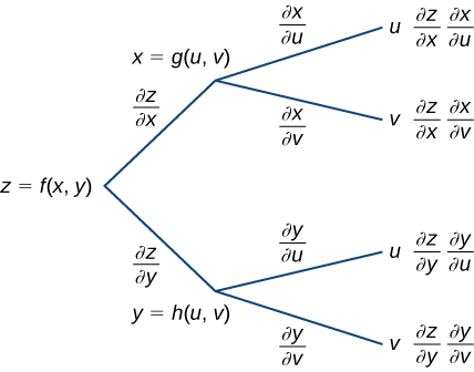
When the intermediate variables depend on two (or more) independent variables, you get partial derivatives on both sides. If $x = x(s,t)$ and $y = y(s,t)$, then:

$\frac{\partial f}{\partial s} = \frac{\partial f}{\partial x}\frac{\partial x}{\partial s} + \frac{\partial f}{\partial y}\frac{\partial y}{\partial s}$

$\frac{\partial f}{\partial t} = \frac{\partial f}{\partial x}\frac{\partial x}{\partial t} + \frac{\partial f}{\partial y}\frac{\partial y}{\partial t}$

The pattern is the same: for each independent variable, sum over all intermediate variables.

Multivariable Calculus Fundamentals

Multivariable Functions and Differentiability

The chain rule formula above requires that $f$ be differentiable at the point in question. A function $f(x,y)$ is differentiable at a point if its partial derivatives exist and are continuous in a neighborhood of that point. (Having partial derivatives exist at a single point is not enough on its own.)

Differentiability guarantees that $f$ can be well-approximated by a linear function near that point:

$f(x_0 + \Delta x,\; y_0 + \Delta y) \approx f(x_0, y_0) + \frac{\partial f}{\partial x}\Delta x + \frac{\partial f}{\partial y}\Delta y$

This linear approximation is exactly the total differential, and it's what makes the chain rule valid. If $f$ is not differentiable, the chain rule formula can fail even when the partial derivatives exist.

Gradient Vector and Jacobian Matrix

The gradient vector packages all partial derivatives of a scalar-valued function into one object:

$\nabla f = \left(\frac{\partial f}{\partial x_1},\; \frac{\partial f}{\partial x_2},\; \ldots,\; \frac{\partial f}{\partial x_n}\right)$

It points in the direction of greatest increase of $f$ and its magnitude gives the rate of that increase. The chain rule for a scalar function $f$ composed with a path $\mathbf{r}(t)$ can be written compactly as $\frac{df}{dt} = \nabla f \cdot \mathbf{r}'(t)$.

When the outer function is vector-valued, the gradient generalizes to the Jacobian matrix. For $\mathbf{f}(x_1, \ldots, x_n) = (f_1, f_2, \ldots, f_m)$, the Jacobian is the $m \times n$ matrix whose $(i, j)$-entry is $\frac{\partial f_i}{\partial x_j}$:

$J_{\mathbf{f}} = \begin{pmatrix} \frac{\partial f_1}{\partial x_1} & \cdots & \frac{\partial f_1}{\partial x_n} \\ \vdots & \ddots & \vdots \\ \frac{\partial f_m}{\partial x_1} & \cdots & \frac{\partial f_m}{\partial x_n} \end{pmatrix}$

The most general form of the multivariable chain rule is then matrix multiplication of Jacobians. If $\mathbf{f}$ maps $\mathbb{R}^n \to \mathbb{R}^m$ and $\mathbf{g}$ maps $\mathbb{R}^p \to \mathbb{R}^n$, then:

$J_{\mathbf{f} \circ \mathbf{g}} = J_{\mathbf{f}} \cdot J_{\mathbf{g}}$

Every version of the chain rule you'll encounter in this course (scalar with one parameter, scalar with several parameters, vector-valued compositions) is a special case of this single matrix equation. When you're unsure how to set up a chain rule problem, writing out the Jacobians and multiplying them will always give the correct answer.