3.1 Definition and computation of partial derivatives

Partial Derivatives and Multivariable Functions

Partial derivatives let you isolate how a multivariable function changes with respect to one variable while holding everything else constant. They're the foundation for nearly everything else in Calculus IV: tangent planes, optimization, gradient fields, and more.

Definition and Notation of Partial Derivatives

A multivariable function depends on two or more independent variables. For example, $f(x, y) = x^2 + y^2$ takes in two inputs and returns a single output.

A partial derivative measures the rate of change of such a function with respect to one variable, treating all other variables as constants. Think of it this way: if you're standing on a surface $z = f(x, y)$ and you walk purely in the $x$-direction, the partial derivative $\frac{\partial f}{\partial x}$ tells you how steeply the surface rises or falls along that path.

The symbol $\partial$ (as opposed to $d$) signals that other variables are being held fixed. Common notations you'll see:

• $\frac{\partial f}{\partial x}$ or $f_x$ for the partial derivative with respect to $x$
• $\frac{\partial f}{\partial y}$ or $f_y$ for the partial derivative with respect to $y$

The formal limit definition mirrors single-variable calculus:

$f_x(a, b) = \lim_{h \to 0} \frac{f(a + h,\, b) - f(a, b)}{h}$

Notice only the $x$-input changes; $y$ stays at $b$.

Computing Partial Derivatives

The mechanics are straightforward: differentiate with respect to your target variable using all the standard rules (power, product, chain, trig, etc.), and treat every other variable as if it were a constant number.

Step-by-step process:

1. Identify which variable you're differentiating with respect to.
2. Mentally replace every other variable with a constant (some students find it helpful to literally substitute a letter like $k$ for the held-fixed variable while computing).
3. Differentiate using the usual single-variable rules.
4. Substitute the original variable names back in if you replaced them.

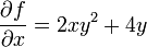
Example 1: Let $f(x, y) = x^2 y$.

• For $\frac{\partial f}{\partial x}$: treat $y$ as a constant. You're differentiating $y \cdot x^2$, which gives $2xy$.
• For $\frac{\partial f}{\partial y}$: treat $x$ as a constant. You're differentiating $x^2 \cdot y$, which gives $x^2$.

Example 2: Let $f(x, y) = x^3 + 2xy + \sin(y)$.

• $\frac{\partial f}{\partial x} = 3x^2 + 2y$ (the $\sin(y)$ term is a constant with respect to $x$, so it vanishes)
• $\frac{\partial f}{\partial y} = 2x + \cos(y)$ (the $x^3$ term vanishes since it's constant with respect to $y$)

A common early mistake is forgetting to zero out terms that don't involve your target variable. If a term has no $x$ in it, its partial derivative with respect to $x$ is zero.

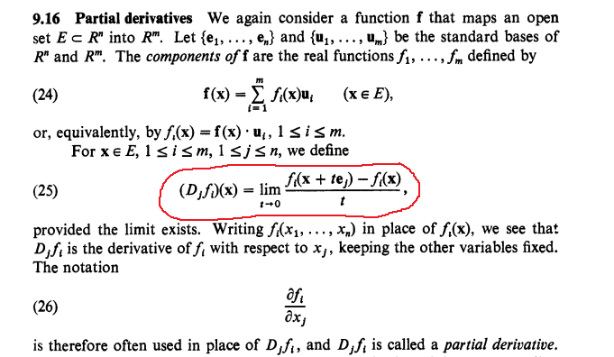
Higher-Order Partial Derivatives

Just as in single-variable calculus, you can differentiate again. Second-order partial derivatives come in two flavors:

• Unmixed: differentiate twice with respect to the same variable, e.g., $f_{xx} = \frac{\partial^2 f}{\partial x^2}$
• Mixed: differentiate with respect to different variables, e.g., $f_{xy} = \frac{\partial^2 f}{\partial y \, \partial x}$

Be careful with the notation for mixed partials. In $\frac{\partial^2 f}{\partial y \, \partial x}$, you differentiate with respect to $x$ first, then with respect to $y$ (right to left). In subscript notation $f_{xy}$, you go left to right: $x$ first, then $y$. These conventions are opposite, which trips people up.

Clairaut's Theorem and Mixed Partial Derivatives

Clairaut's theorem says: if $f_{xy}$ and $f_{yx}$ are both continuous near a point, then $f_{xy} = f_{yx}$ at that point. In practice, this means the order of differentiation doesn't matter for the vast majority of functions you'll encounter in this course.

Example: Let $f(x, y) = x^2y + xy^2$.

1. Compute $f_x = 2xy + y^2$, then $f_{xy} = \frac{\partial}{\partial y}(2xy + y^2) = 2x + 2y$.
2. Compute $f_y = x^2 + 2xy$, then $f_{yx} = \frac{\partial}{\partial x}(x^2 + 2xy) = 2x + 2y$.

Both mixed partials equal $2x + 2y$, confirming Clairaut's theorem. If you ever compute them and get different results, check your algebra first.

Geometric Interpretation

Tangent Planes and Directional Derivatives

Partial derivatives have a clean geometric meaning. The partial derivative $f_x(a, b)$ is the slope of the curve you get by slicing the surface $z = f(x, y)$ with the plane $y = b$. Similarly, $f_y(a, b)$ is the slope of the slice at $x = a$. Together, these two slopes determine the tangent plane at a point.

The equation of the tangent plane to $z = f(x, y)$ at the point $(a, b, f(a, b))$ is:

$z - f(a, b) = f_x(a, b)(x - a) + f_y(a, b)(y - b)$

This is the best linear approximation to the surface near that point, and it generalizes the tangent line from Calc I.

The directional derivative extends partial derivatives beyond just the $x$- and $y$-directions. It measures the rate of change of $f$ at $(a, b)$ in the direction of any unit vector $\vec{u} = \langle u_1, u_2 \rangle$:

$D_{\vec{u}}f(a, b) = f_x(a, b)\, u_1 + f_y(a, b)\, u_2$

Note that $\vec{u}$ must be a unit vector. If you're given a direction that isn't unit length, normalize it first.

The gradient vector $\nabla f(a, b) = \langle f_x(a, b),\, f_y(a, b) \rangle$ packages both partial derivatives into a single vector. Two key facts about the gradient:

• It points in the direction of the greatest rate of increase of $f$.
• It's perpendicular to the level curves of $f$ at that point.

Example: For $f(x, y) = x^2 + y^2$, the gradient at $(a, b)$ is $\nabla f = \langle 2a, 2b \rangle$. The level curves are circles centered at the origin, and $\nabla f$ points radially outward, perpendicular to those circles, exactly as expected.