Critical Points and Partial Derivatives
Identifying Critical Points
A critical point of a multivariable function is a point where all partial derivatives are simultaneously zero or where at least one partial derivative is undefined. These are the only locations where a function can achieve a local maximum or minimum, so finding them is the first step in any optimization problem.
To find critical points of a function :
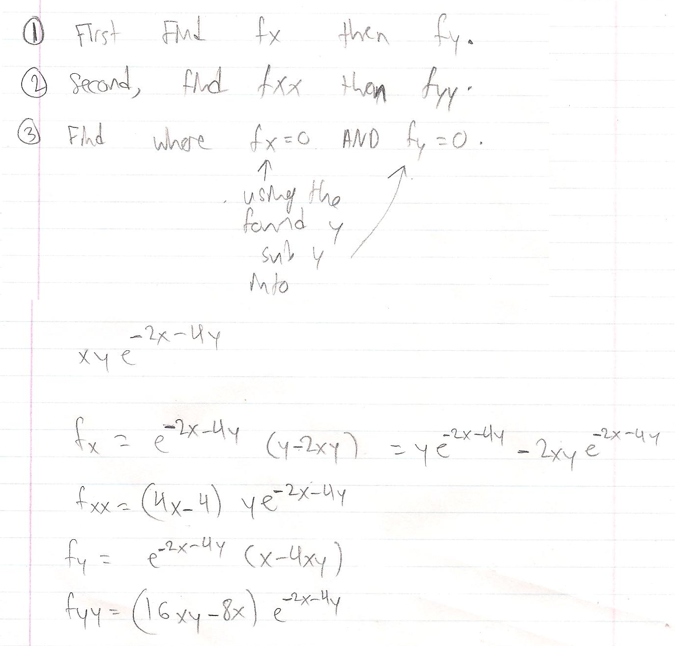
- Compute and .
- Set both partial derivatives equal to zero: and .
- Solve the resulting system of equations simultaneously for and .
Not every critical point is a max or min. Some turn out to be saddle points, where the function increases in certain directions and decreases in others. That's why classification (covered below) matters.
Gradient Vector and Its Role
The gradient vector packages the partial derivatives into a single vector. It points in the direction of steepest ascent of the function at any given point.
- At a critical point, . The function has no single "steepest" direction there, which is exactly why these points are candidates for extrema.
- The gradient is always perpendicular to the level curves (or level surfaces) of . This geometric fact becomes important in constrained optimization later.
- The magnitude tells you how steeply the function is changing. A larger magnitude means a steeper slope.

Classifying Critical Points
The Hessian Matrix
Once you've found a critical point, you need to determine what kind it is. The tool for this is the Hessian matrix, a square matrix of all second-order partial derivatives.
For , the Hessian is:
The quantity that drives classification is the determinant of the Hessian, often written or :
Note that by Clairaut's theorem, whenever the second partials are continuous, so you only need to compute once.
Second Derivative Test
With the determinant evaluated at a critical point , classification works as follows:
-
Compute , , and .
-
Calculate .
-
Classify the critical point:
- and → local minimum (the surface curves upward in every direction, like a valley)
- and → local maximum (the surface curves downward in every direction, like a hilltop)
- → saddle point (the surface curves up in some directions and down in others, like a mountain pass)
- → test is inconclusive; you'll need other methods (such as analyzing the function's behavior directly)
A common mistake is forgetting the case. The test genuinely tells you nothing here. Don't assume it's a saddle point just because it isn't clearly a max or min.
Why the Test Works (Intuition)
The sign of captures whether the second-order behavior is consistent across directions. When , the surface bends the same way (both up or both down) along every direction through the critical point, so alone tells you which. When , the surface bends up along one direction and down along another, producing the characteristic saddle shape. This connects directly to the eigenvalues of the Hessian: means both eigenvalues share the same sign, while means they have opposite signs.