17.3 Flow lines and equilibrium points

Flow Lines and Equilibrium Points

Vector fields assign a vector to each point in some region of space. Flow lines and equilibrium points give you the tools to understand how things move through those fields. Flow lines trace the paths particles follow, and equilibrium points mark where motion stops entirely. Together, they form the backbone of phase plane analysis, connecting vector calculus to dynamical systems in areas like fluid flow, orbital mechanics, and population modeling.

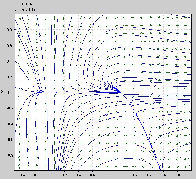
Flow Lines and Trajectories

Graphical Representations of Vector Fields

A flow line (also called an integral curve or streamline) is a curve whose tangent vector at every point equals the vector field at that point. If you dropped a particle into the field, the flow line is the path it would trace out.

Formally, a flow line for a vector field $\mathbf{F}(x, y)$ is a parametric curve $\mathbf{r}(t) = (x(t), y(t))$ satisfying:

$\frac{d\mathbf{r}}{dt} = \mathbf{F}(\mathbf{r}(t))$

This means $\frac{dx}{dt} = F_1(x, y)$ and $\frac{dy}{dt} = F_2(x, y)$, where $F_1$ and $F_2$ are the component functions of the field.

A trajectory is the specific flow line determined by a particular initial condition $\mathbf{r}(0) = (x_0, y_0)$. Different starting points yield different trajectories through the same vector field.

A phase portrait collects many trajectories (from various initial conditions) into a single diagram. It gives you a global picture of the system's behavior: where trajectories converge, diverge, spiral, or form closed loops.

Interpreting Flow Lines and Trajectories

The spacing and arrangement of flow lines encode information about the field:

• Closely spaced flow lines indicate regions where the field has large magnitude, meaning particles move quickly there.
• Widely spaced flow lines correspond to regions of small magnitude and slower movement.
• Flow lines for a smooth vector field never cross each other (by the uniqueness theorem for ODEs). If two flow lines appear to meet at a point, that point is an equilibrium where the field vanishes. Near such points, trajectories may converge, diverge, or change direction, revealing the system's long-term behavior.

Equilibrium Points

Types of Equilibrium Points

An equilibrium point (also called a fixed point or critical point) is a location $(x^*, y^*)$ where the vector field is zero:

$\mathbf{F}(x^*, y^*) = \mathbf{0}$

At such a point, a particle placed there would remain stationary. You find equilibrium points by solving $\frac{dx}{dt} = 0$ and $\frac{dy}{dt} = 0$ simultaneously.

Equilibrium points come in several types based on how nearby trajectories behave:

• Sink (stable node or spiral): All nearby trajectories converge toward the equilibrium as $t \to \infty$. Think of a ball settling to the bottom of a bowl.
• Source (unstable node or spiral): All nearby trajectories move away from the equilibrium as $t \to \infty$. This is like a ball balanced on top of a hill.
• Saddle point: Trajectories approach along one direction but are repelled along another. The equilibrium is unstable overall because almost all nearby trajectories eventually move away.

Identifying Equilibrium Points

There are two complementary approaches:

Algebraically:

1. Write out the system: $\frac{dx}{dt} = F_1(x,y)$ and $\frac{dy}{dt} = F_2(x,y)$.
2. Set both $F_1(x,y) = 0$ and $F_2(x,y) = 0$.
3. Solve the resulting system of equations for all $(x^*, y^*)$ pairs.

Graphically using nullclines:

• The $x$-nullcline is the set of points where $\frac{dx}{dt} = 0$ (horizontal arrows in the phase portrait).
• The $y$-nullcline is the set of points where $\frac{dy}{dt} = 0$ (vertical arrows in the phase portrait).
• Equilibrium points occur exactly where these nullclines intersect, since both components of the field are zero there.

Nullclines are also useful beyond just finding equilibria: they divide the phase plane into regions where you can determine the sign of each component, giving you the general direction of flow in each region.

Stability of Equilibrium Points

Determining Stability

To classify an equilibrium point rigorously, you linearize the system near that point and examine the resulting linear system's behavior.

Step-by-step process:

1. Find the Jacobian matrix of the system. For $\mathbf{F} = (F_1, F_2)$:

$J(x,y) = \begin{pmatrix} \frac{\partial F_1}{\partial x} & \frac{\partial F_1}{\partial y} \\ \frac{\partial F_2}{\partial x} & \frac{\partial F_2}{\partial y} \end{pmatrix}$

1. Evaluate $J$ at the equilibrium point $(x^*, y^*)$.

2. Compute the eigenvalues $\lambda_1, \lambda_2$ of $J(x^*, y^*)$, typically by solving:

$\det(J - \lambda I) = 0$

This gives a characteristic equation $\lambda^2 - \tau\lambda + \Delta = 0$, where $\tau = \text{tr}(J)$ and $\Delta = \det(J)$.

1. Read off the stability from the eigenvalues:
   • Both eigenvalues have negative real parts → stable (sink)
   • Both eigenvalues have positive real parts → unstable (source)
   • Eigenvalues have real parts of opposite sign → saddle point

Classifying Equilibrium Points

The eigenvalues tell you not just stability but the geometric character of the equilibrium:

A few things worth noting:

• Centers are classified as stable in the sense that trajectories don't leave the neighborhood, but they're not asymptotically stable since trajectories never actually reach the equilibrium. The linearization can also be misleading here: nonlinear terms may turn a center into a spiral.
• Repeated eigenvalues require extra care. If the Jacobian is diagonalizable, you get a star node (trajectories approach straight in from all directions). If not, you get an improper node with a single dominant direction.
• The trace-determinant plane offers a quick visual shortcut: plotting $\tau = \text{tr}(J)$ against $\Delta = \det(J)$ immediately tells you the classification without computing eigenvalues explicitly. The parabola $\tau^2 - 4\Delta = 0$ separates nodes from spirals, the $\Delta$-axis separates stable from unstable, and $\Delta < 0$ gives saddle points.