8.2 The method of Lagrange multipliers

Lagrange Multipliers and Lagrangian Function

Lagrange Multiplier and Lagrangian Function

The Lagrange multiplier $\lambda$ is a variable we introduce to convert a constrained optimization problem into an unconstrained one. Instead of trying to optimize $f$ while separately enforcing a constraint, we fold everything into a single function and optimize that.

The Lagrangian function $L$ combines the objective function $f(x, y)$ with the constraint $g(x, y) = 0$ using the multiplier:

$L(x, y, \lambda) = f(x, y) - \lambda \, g(x, y)$

Note the sign convention: some textbooks write $f + \lambda g$ and others write $f - \lambda g$. Both work because $\lambda$ can absorb the sign. Just be consistent with whatever your course uses. The guide below uses the $f - \lambda g$ convention, but the worked example keeps the $+\lambda g$ form to match a common presentation. Watch your professor's notes.

Example: Minimize $f(x, y) = x^2 + y^2$ subject to $g(x, y) = x + y - 1 = 0$.

Using the $+\lambda g$ convention here:

$L(x, y, \lambda) = x^2 + y^2 + \lambda(x + y - 1)$

Critical Points and the Lagrange Multiplier Theorem

To find the critical points of the Lagrangian, set all of its partial derivatives equal to zero:

1. $\frac{\partial L}{\partial x} = 0$
2. $\frac{\partial L}{\partial y} = 0$
3. $\frac{\partial L}{\partial \lambda} = 0$

Condition 3 simply recovers the original constraint $g(x, y) = 0$. Conditions 1 and 2 enforce the gradient relationship (more on that below). Solving this system simultaneously gives you the critical points $(x, y, \lambda)$.

Lagrange Multiplier Theorem: If $(x_0, y_0)$ is a local extremum of $f(x, y)$ subject to $g(x, y) = 0$, and $\nabla g(x_0, y_0) \neq \mathbf{0}$, then there exists a scalar $\lambda_0$ such that $(x_0, y_0, \lambda_0)$ is a critical point of the Lagrangian. This is a necessary condition, not sufficient on its own.

Continuing the example:

1. $\frac{\partial L}{\partial x} = 2x + \lambda = 0 \implies \lambda = -2x$
2. $\frac{\partial L}{\partial y} = 2y + \lambda = 0 \implies \lambda = -2y$
3. $\frac{\partial L}{\partial \lambda} = x + y - 1 = 0$

From steps 1 and 2: $-2x = -2y$, so $x = y$. Substituting into step 3: $2x = 1$, giving $x = y = \frac{1}{2}$ and $\lambda = -1$.

The single critical point is $\left(\frac{1}{2},\, \frac{1}{2}\right)$ with $\lambda = -1$, and $f\!\left(\frac{1}{2}, \frac{1}{2}\right) = \frac{1}{2}$. Since $f = x^2 + y^2$ can grow without bound on the line $x + y = 1$, this point is the constrained minimum.

Gradient Vectors and Parallel Gradients

Gradient Vectors and Parallel Gradients

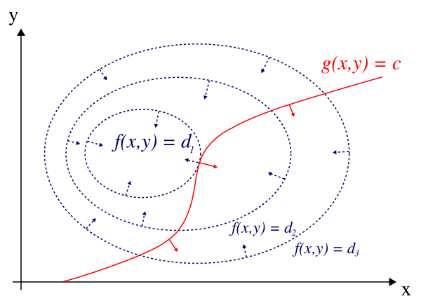
The gradient $\nabla f(x, y) = \left(\frac{\partial f}{\partial x},\, \frac{\partial f}{\partial y}\right)$ points perpendicular to the level curves of $f$. Similarly, $\nabla g$ points perpendicular to the constraint curve $g(x, y) = 0$.

At a constrained extremum, the level curve of $f$ is tangent to the constraint curve. That tangency means the two gradient vectors must be parallel:

$\nabla f(x_0, y_0) = \lambda \, \nabla g(x_0, y_0)$

This is the geometric heart of the method. If the gradients weren't parallel, you could slide along the constraint and still increase (or decrease) $f$, so you wouldn't be at an extremum.

First-Order Necessary and Second-Order Sufficient Conditions

First-order necessary conditions for $(x_0, y_0)$ to be a constrained extremum:

1. $g(x_0, y_0) = 0$ (the point lies on the constraint)
2. $\nabla f(x_0, y_0) = \lambda \, \nabla g(x_0, y_0)$ for some scalar $\lambda$

These conditions find candidates but don't tell you whether each candidate is a max, min, or neither.

Second-order sufficient conditions classify those candidates. The standard tool is the bordered Hessian. For one constraint in two variables, the bordered Hessian is:

$\bar{H} = \begin{vmatrix} 0 & g_x & g_y \\ g_x & L_{xx} & L_{xy} \\ g_y & L_{xy} & L_{yy} \end{vmatrix}$

where all partial derivatives are evaluated at the critical point.

• If $\det(\bar{H}) > 0$, the point is a constrained maximum.
• If $\det(\bar{H}) < 0$, the point is a constrained minimum.

For problems with more variables, you extend the bordered Hessian and check a sequence of determinants (the bordered leading principal minors). Your course may also frame this in terms of the eigenvalues of the Hessian of $L$ restricted to the tangent space of the constraint.

Constrained Optimization

Saddle Points and Multiple Constraints

Saddle points are critical points of the Lagrangian that are neither constrained maxima nor constrained minima. At a saddle point, $f$ increases in some directions along the constraint surface and decreases in others. The bordered Hessian test is inconclusive (determinant equals zero) or the eigenvalue pattern is mixed.

Multiple Constraints

When you have more than one constraint, introduce a separate multiplier for each. For constraints $g_1(x, y) = 0,\; g_2(x, y) = 0,\; \ldots,\; g_m(x, y) = 0$:

$L(x, y, \lambda_1, \ldots, \lambda_m) = f(x, y) + \lambda_1 g_1(x, y) + \lambda_2 g_2(x, y) + \cdots + \lambda_m g_m(x, y)$

The first-order conditions become:

$\nabla f = \lambda_1 \nabla g_1 + \lambda_2 \nabla g_2 + \cdots + \lambda_m \nabla g_m$

along with each constraint $g_i = 0$. An important regularity requirement: the gradient vectors $\nabla g_1, \nabla g_2, \ldots, \nabla g_m$ must be linearly independent at the solution. If they aren't, the method can fail.

Example: Minimize $f(x, y) = x^2 + y^2$ subject to $g_1 = x + y - 1 = 0$ and $g_2 = x - y - 1 = 0$.

$L = x^2 + y^2 + \lambda_1(x + y - 1) + \lambda_2(x - y - 1)$

Before even differentiating, notice that the two constraints together force $x + y = 1$ and $x - y = 1$, which gives $x = 1,\; y = 0$ as the only feasible point. With a single feasible point, there's nothing to optimize over: $f(1, 0) = 1$ is both the min and the max on the feasible set. This illustrates that with enough constraints, the feasible set can shrink to a single point (or even be empty).