1.2 Vector-valued functions and their derivatives

Vector-Valued Functions and Parametric Equations

A vector-valued function takes a real number (usually $t$) as input and outputs a vector. This gives you a way to describe curves and trajectories in 2D or 3D space, where the parameter $t$ often represents time. If you've worked with parametric equations before, vector-valued functions are the natural vector packaging of that same idea.

Representing Curves and Motion with Vector-Valued Functions

A vector-valued function maps real numbers to vectors in two or three-dimensional space. For a 3D function:

$\vec{r}(t) = \langle f(t), g(t), h(t) \rangle$

The individual pieces $f(t)$, $g(t)$, and $h(t)$ are called component functions. Each one is a regular scalar-valued function that tracks the object's position along a single axis ($x$, $y$, or $z$) as $t$ changes.

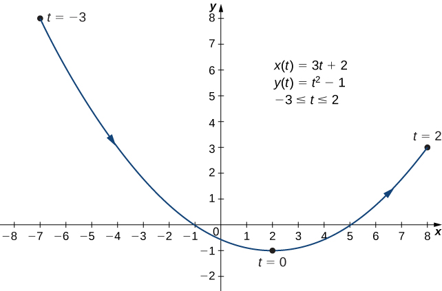
This connects directly to parametric equations. For a curve in 2D, the parametric equations $x = f(t)$ and $y = g(t)$ are exactly the component functions of $\vec{r}(t) = \langle f(t), g(t) \rangle$. The vector-valued function just bundles those parametric equations into one compact object.

• Parametric/vector representations can describe curves that fail the vertical line test, like circles or figure-eights, which you can't write as $y = f(x)$
• The parameter $t$ doesn't have to represent time, but it very often does in physics applications

Graphing and Evaluating Vector-Valued Functions

To graph a vector-valued function, you trace out the curve by plotting the terminal points of $\vec{r}(t)$ for various values of $t$:

1. Choose several values of $t$ across your domain.
2. Plug each into the component functions to get coordinate points $(f(t), g(t))$ or $(f(t), g(t), h(t))$.
3. Plot those points and connect them in order of increasing $t$.

For example, $\vec{r}(t) = \langle \cos(t), \sin(t) \rangle$ with $t \in [0, 2\pi]$ traces out a unit circle centered at the origin. The direction of increasing $t$ gives the curve an orientation (counterclockwise, in this case).

Evaluating at a specific $t$-value just means substituting into each component. For $\vec{r}(t) = \langle t^2, t, t^3 \rangle$:

$\vec{r}(2) = \langle 4, 2, 8 \rangle$

This output is a position vector pointing from the origin to the point $(4, 2, 8)$.

Limits and Continuity

Limits of Vector-Valued Functions

The key principle here is simple: everything works component-wise. To take the limit of a vector-valued function, take the limit of each component separately.

$\lim_{t \to a} \vec{r}(t) = \left\langle \lim_{t \to a} f(t),\; \lim_{t \to a} g(t),\; \lim_{t \to a} h(t) \right\rangle$

The vector limit exists if and only if every component limit exists. You use all the same limit techniques you already know from single-variable calculus (factoring, L'Hôpital's rule, etc.) on each component.

Example: For $\vec{r}(t) = \left\langle \frac{t^2 - 1}{t - 1},\; \frac{t^3 - 1}{t - 1} \right\rangle$, find $\lim_{t \to 1} \vec{r}(t)$:

• First component: $\frac{t^2 - 1}{t - 1} = \frac{(t-1)(t+1)}{t-1} = t + 1 \to 2$
• Second component: $\frac{t^3 - 1}{t - 1} = \frac{(t-1)(t^2+t+1)}{t-1} = t^2 + t + 1 \to 3$

So $\lim_{t \to 1} \vec{r}(t) = \langle 2, 3 \rangle$.

Continuity of Vector-Valued Functions

A vector-valued function $\vec{r}(t)$ is continuous at $t = a$ if:

$\lim_{t \to a} \vec{r}(t) = \vec{r}(a)$

Again, this reduces to checking each component. If all component functions are continuous at $t = a$, then $\vec{r}(t)$ is continuous there. Geometrically, continuity means the curve has no breaks or jumps.

For instance, $\vec{r}(t) = \langle \sin(t), \cos(t) \rangle$ is continuous for all $t$ because both $\sin(t)$ and $\cos(t)$ are continuous everywhere. On the other hand, if any single component has a discontinuity at some $t = a$, the entire vector-valued function is discontinuous there.

Derivatives and Applications

Derivatives of Vector-Valued Functions

Differentiation also works component-wise. For $\vec{r}(t) = \langle f(t), g(t), h(t) \rangle$:

$\vec{r}'(t) = \langle f'(t),\; g'(t),\; h'(t) \rangle$

You differentiate each component using the same rules from single-variable calculus (power rule, chain rule, product rule, etc.).

What does the derivative mean geometrically? The vector $\vec{r}'(t)$ is tangent to the curve at the point $\vec{r}(t)$, and it points in the direction of increasing $t$. This is worth remembering because it comes up constantly in later topics like unit tangent vectors and curvature.

Example: For $\vec{r}(t) = \langle t^2, \sin(t), e^t \rangle$:

$\vec{r}'(t) = \langle 2t, \cos(t), e^t \rangle$

At $t = 0$, the tangent vector is $\vec{r}'(0) = \langle 0, 1, 1 \rangle$.

Velocity and Acceleration Vectors

When $\vec{r}(t)$ represents the position of a moving object, its derivatives have direct physical meaning:

• Velocity: $\vec{v}(t) = \vec{r}'(t)$. This gives the instantaneous velocity as a vector (direction and magnitude).
• Speed: $\|\vec{v}(t)\| = \|\vec{r}'(t)\|$. Speed is the magnitude of velocity, always a non-negative scalar.
• Acceleration: $\vec{a}(t) = \vec{v}'(t) = \vec{r}''(t)$. This tells you how the velocity vector is changing over time.

Note that acceleration doesn't just mean "speeding up." The acceleration vector can change the direction of motion, the speed, or both.

Example: A particle moves along $\vec{r}(t) = \langle \cos(t), \sin(t), t \rangle$ (a helix spiraling upward).

1. Velocity: $\vec{v}(t) = \langle -\sin(t), \cos(t), 1 \rangle$
2. Speed: $\|\vec{v}(t)\| = \sqrt{\sin^2(t) + \cos^2(t) + 1} = \sqrt{2}$, which is constant
3. Acceleration: $\vec{a}(t) = \langle -\cos(t), -\sin(t), 0 \rangle$

The speed is constant at $\sqrt{2}$, yet the acceleration is nonzero. That's because the acceleration here is purely changing the direction of motion (the circular part), not the speed. This distinction between changing speed and changing direction is something you'll revisit when you study tangential and normal components of acceleration.