📘Intermediate Algebra Unit 8 Review
8.7 Use Radicals in Functions
8.7 Use Radicals in Functions
Unit & Topic Study Guides
Foundations
Solving Linear Equations
Graphs and Functions
Systems of Linear Equations
Polynomials and Polynomial Functions
Factoring
Rational Expressions and Functions
Roots and Radicals
Quadratic Equations and Functions
Exponential & Logarithmic Functions
Conics
Sequences, Series & Binomial Theorem
Radicals in Functions
Radical functions are functions that contain a root expression, like a square root or cube root. Working with them means you need to think carefully about what inputs are allowed (the domain), how to evaluate them, and what their graphs look like.
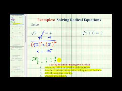
Solving Radical Functions
To evaluate a radical function at a specific input, substitute the value into the function and simplify.
Steps:
- Replace the variable with the given input value everywhere it appears.
- Simplify the expression under the radical (the radicand) first.
- Evaluate the root.
Example: For , find .
- Replace with 3:
- Simplify the radicand:
- Evaluate:
A few notes on different root types:
- Square roots always give the principal (non-negative) root. So , not .
- Cube roots can output any real number, including negatives. For example, .
- Higher-order roots (4th, 5th, etc.) follow the same even/odd pattern: even-index roots require non-negative radicands, odd-index roots accept anything.
Domain of Radical Functions
The domain is the set of all input values where the function produces a real number output. The key rule depends on whether the root's index is even or odd.
Even-index radicals (square roots, 4th roots, etc.): the radicand must be greater than or equal to zero. You can't take the square root of a negative number and get a real result.
Example: Find the domain of .
-
Set the radicand :
-
Solve:
-
Domain:
Odd-index radicals (cube roots, 5th roots, etc.): the domain is all real numbers, because you can take an odd root of any number.
Example: has domain .
Also watch for additional restrictions. If the radical is part of a fraction, you still need to exclude values that make the denominator zero. For instance, requires (strictly greater than, since in the denominator gives division by zero), so the domain is .
Graphs of Radical Functions
Graphing a radical function follows a straightforward process.
- Find the domain so you know which -values are valid.
- Build a table of points by choosing -values that produce clean results (perfect squares for square root functions, perfect cubes for cube root functions, etc.).
- Plot the points and connect them with a smooth curve.
Example: Graph .
- Domain:
- Choose strategic -values:
| 0 | 0 |
| 1 | 1 |
| 4 | 2 |
| 9 | 3 |
- Plot (0, 0), (1, 1), (4, 2), (9, 3) and draw a smooth curve through them.
Notice the curve starts at the origin and rises gradually, getting flatter as increases. This "slowing down" shape is typical of square root functions.
Key features to identify on any radical graph:
- Starting point: where the curve begins (determined by the domain restriction)
- x-intercept(s): where the graph crosses the x-axis ()
- y-intercept: where the graph crosses the y-axis (), if that value is in the domain
- Increasing or decreasing: whether the function rises or falls as increases
- Range: the set of all output values. For , the range is
Functions, Graphs, and Inequalities
A function assigns exactly one output to each input. The graph of a radical function shows all its input-output pairs visually, which makes it easier to read off the domain and range.
Radical inequalities ask you to find the -values where a radical expression is greater than, less than, or equal to some value.
Example: Solve .
- Square both sides:
- Solve:
- Check the domain: requires , so . Since already satisfies this, the solution is .
Be careful when squaring both sides of an inequality. Squaring is only safe here because both sides are non-negative (a square root is always , and 3 is positive). If either side could be negative, you'd need to handle the problem differently.