10.2 Evaluate and Graph Exponential Functions

Exponential functions model situations where a quantity grows or shrinks at a rate proportional to its current value. They show up constantly in problems involving population growth, compound interest, and radioactive decay, so getting comfortable with their form and behavior is essential for the rest of this course.

Exponential Functions

Key features of exponential graphs

The general form of an exponential function is $f(x) = ab^x$.

• $a$ is the initial value (the y-intercept). When $x = 0$, you get $f(0) = a \cdot b^0 = a$, so the graph always passes through $(0, a)$.
• $b$ is the base, and it controls whether the function grows or decays:
  • If $b > 1$, the function shows exponential growth. Each time $x$ increases by 1, the output multiplies by $b$. For example, $f(x) = 3(2)^x$ doubles with every step.
  • If $0 < b < 1$, the function shows exponential decay. The output shrinks by a factor of $b$ with each step. For example, $f(x) = 100(0.5)^x$ cuts in half each time $x$ increases by 1.
  • The base $b$ must be positive and cannot equal 1 (since $1^x = 1$ for all $x$, which is just a constant).

Graphing tips:

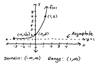
1. Plot the y-intercept $(0, a)$.
2. Pick a couple of $x$-values (like $x = 1$ and $x = -1$) and compute $f(x)$ to get additional points.
3. Draw a smooth curve through the points.
4. Sketch the horizontal asymptote at $y = 0$. The graph approaches this line but never touches it.

For growth ($b > 1$): the curve rises steeply to the right and flattens out toward $y = 0$ on the left. For decay ($0 < b < 1$): the curve falls toward $y = 0$ on the right and rises steeply to the left.

Domain and range:

• The domain is all real numbers: $(-\infty, \infty)$.
• The range depends on the sign of $a$:
  • If $a > 0$, the range is $(0, \infty)$ (outputs are always positive).
  • If $a < 0$, the range is $(-\infty, 0)$ (the graph is reflected below the x-axis, and outputs are always negative).

Properties of exponential functions

• Exponential functions are continuous, meaning their graphs have no breaks, holes, or jumps.
• They are monotonic: if $b > 1$, the function is always increasing; if $0 < b < 1$, it's always decreasing. This means exponential functions are one-to-one, so every output corresponds to exactly one input.
• Because they're one-to-one, exponential functions have inverses. The inverse of an exponential function is a logarithmic function. This relationship is the foundation of the next section on logarithms.

Solving exponential equations

Method 1: Same base (algebraic approach)

If you can rewrite both sides of the equation with the same base, set the exponents equal and solve.

1. Rewrite each side as a power of the same base.
2. Since $b^m = b^n$ implies $m = n$, set the exponents equal.
3. Solve the resulting equation.

This also works when you need to convert bases. For instance, to solve $4^x = 8$, rewrite as $(2^2)^x = 2^3$, giving $2^{2x} = 2^3$, so $2x = 3$ and $x = \frac{3}{2}$.

Method 2: Using logarithms

When you can't easily match bases, take a logarithm of both sides.

1. Isolate the exponential expression on one side.
2. Take the logarithm of both sides (common log or natural log both work).
3. Use the power rule $\log(b^x) = x\log(b)$ to bring the exponent down.
4. Solve for the variable.

Applications of exponential models

Growth and decay formulas

The continuous growth/decay model uses Euler's number $e \approx 2.718$:

$A(t) = A_0 e^{kt}$

• $A_0$ is the initial amount (at $t = 0$).
• $k$ is the continuous rate. If $k > 0$, the model describes growth. If $k < 0$, it describes decay.
• $t$ is time.

Interpreting the rate $k$:

A larger absolute value of $k$ means faster change. For instance, bacteria with $k = 0.35$ per hour grow much faster than a population with $k = 0.02$ per year.

Half-life and doubling time both use the same formula structure:

• Doubling time (growth): $t_{\text{double}} = \frac{\ln(2)}{k}$
• Half-life (decay): $t_{1/2} = \frac{\ln(2)}{|k|}$

Common applications:

• Population growth: modeling how a city or species grows over time
• Compound interest: $A = Pe^{rt}$ for continuously compounded interest, where $P$ is principal and $r$ is the annual rate
• Radioactive decay: determining how long until a substance drops to a safe level
• Newton's Law of Cooling: predicting how quickly an object's temperature approaches room temperature