3.4 Graph Linear Inequalities in Two Variables

Graphing Linear Inequalities in Two Variables

Linear inequalities in two variables divide the coordinate plane into regions, with one region representing the solution set. Graphing these inequalities involves drawing a boundary line and shading the correct half-plane based on the inequality symbol and a test point.

This skill matters because many real-world problems involve constraints (budgets, time limits, capacity) rather than exact equations. It also forms the foundation for linear programming, where multiple inequalities create a feasible region used to optimize solutions.

Graphing Linear Inequalities in Two Variables

Verification of two-variable inequality solutions

To check whether a specific point is a solution to a linear inequality, plug its coordinates into the inequality and see if the resulting statement is true or false.

• Substitute the given $x$ and $y$ values into the inequality
• Simplify both sides
• If the statement is true, the point is a solution
• If the statement is false, the point is not a solution

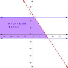
Example: Is $(2, 3)$ a solution to $3x + 2y < 12$?

1. Substitute $x = 2$ and $y = 3$: $3(2) + 2(3) < 12$
2. Simplify: $6 + 6 < 12$, which gives $12 < 12$
3. That's false (12 is not less than 12), so $(2, 3)$ is not a solution

Notice that $(2, 3)$ would satisfy $3x + 2y \leq 12$ since $12 \leq 12$ is true. The difference between $<$ and $\leq$ matters here.

Interpretation of linear inequality graphs

A linear inequality graph splits the coordinate plane into two half-planes separated by a boundary line. Every point in one half-plane satisfies the inequality; every point in the other does not.

Boundary line rules:

• The boundary line comes from replacing the inequality symbol with $=$
• Use a dashed line for strict inequalities ($<$ or $>$) because points on the line are not included in the solution set
• Use a solid line for inclusive inequalities ($\leq$ or $\geq$) because points on the line are included

Shaded region: The shaded side of the boundary line represents the solution set. You determine which side to shade using a test point (covered in the next section).

Graphing of linear inequalities

Follow these steps to graph a linear inequality:

1. Rewrite in slope-intercept form if helpful: get the inequality into the form $y < mx + b$, $y > mx + b$, $y \leq mx + b$, or $y \geq mx + b$

2. Graph the boundary line $y = mx + b$

   • Dashed for $<$ or $>$
   • Solid for $\leq$ or $\geq$

3. Pick a test point that is not on the boundary line. The origin $(0, 0)$ is the easiest choice whenever the line doesn't pass through it.

4. Substitute the test point into the original inequality

   • If the result is true, shade the side that contains the test point
   • If the result is false, shade the opposite side

5. Label the graph with the inequality

Quick shortcut: If you've solved for $y$, the inequality symbol tells you which side to shade. For $y < mx + b$ or $y \leq mx + b$, shade below the line. For $y > mx + b$ or $y \geq mx + b$, shade above the line. The test point method always works as a confirmation.

Real-world applications of linear inequalities

Many real-world constraints translate directly into linear inequalities. The general approach:

1. Define your variables and state what each represents
2. Write the inequality that models the constraint, paying close attention to the direction of the inequality symbol
3. Graph the inequality on the coordinate plane
4. Interpret the solution set in the context of the problem (and note that only non-negative values may make sense)

Example: A company produces products A and B. Product A requires 2 hours and product B requires 3 hours. A maximum of 24 hours is available.

• Let $x$ = number of product A, $y$ = number of product B
• Constraint: $2x + 3y \leq 24$
• The shaded region (including the boundary line) shows all possible production combinations that stay within the 24-hour limit
• Since you can't produce negative quantities, the realistic solution set is limited to the first quadrant where $x \geq 0$ and $y \geq 0$

Linear Programming and Feasible Regions

Linear programming takes this idea further by combining multiple inequalities to optimize an outcome.

• The feasible region is the overlapping area where all constraints are satisfied simultaneously. You find it by graphing every inequality on the same coordinate plane and identifying where the shaded regions overlap.
• The objective function is the expression you want to maximize or minimize (like profit or cost). In the example above, the profit function would be $P = 50x + 75y$.
• The optimal solution is typically found at a vertex (corner point) of the feasible region. You evaluate the objective function at each vertex and compare.

This topic gets developed more fully in later courses, but the graphing skills you're building now are the foundation for it.