4.5 Solve Systems of Equations Using Matrices

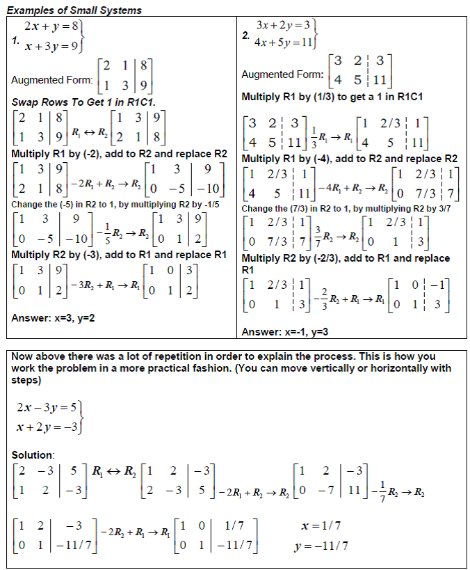
Solving Systems of Equations with Matrices

An augmented matrix is a compact way to represent a system of linear equations so you can solve it using a systematic process called Gaussian elimination. Instead of juggling multiple equations with variables, you organize everything into a grid of numbers and apply row operations until the solution reveals itself.

Augmented Matrices from Equations

To build an augmented matrix, you take each equation in your system and pull out the coefficients and constants, arranging them in rows. A vertical line separates the coefficients (left side) from the constants (right side).

Take this system:

$2x + 3y = 5$ $4x - y = 3$

The augmented matrix looks like this:

$\begin{bmatrix} 2 & 3 & | & 5 \\ 4 & -1 & | & 3 \end{bmatrix}$

• Row 1 holds the coefficients and constant from the first equation: 2, 3, and 5
• Row 2 holds them from the second equation: 4, -1, and 3
• The variables themselves disappear. You just need to keep the coefficients in the same column order ($x$ first, $y$ second) for every row

If a variable is missing from an equation, use 0 as its coefficient. For example, if an equation is $3x = 9$, the row would be $[3 \quad 0 \quad | \quad 9]$ because the $y$-coefficient is 0.

Row Operations for Matrix Simplification

Once you have the augmented matrix, you simplify it using row operations. There are exactly three moves you're allowed to make:

• Row switching: Swap the positions of two rows
• Row multiplication: Multiply every entry in a row by a non-zero constant
• Row addition: Add a multiple of one row to another row (and replace that row with the result)

These operations change the appearance of the matrix but never change the solution to the system. They're the matrix equivalent of the moves you already know from solving equations (multiplying both sides by a constant, adding equations together, etc.).

The goal is to reach row echelon form, where:

• The leading entry (first non-zero number from the left) of each row is strictly to the right of the leading entry in the row above
• All entries below each leading entry are zeros

This staircase-like pattern makes back-substitution straightforward. The process of using row operations to get there is called Gaussian elimination.

Solving a System Step by Step

Here's the full process from start to finish:

1. Write the augmented matrix from the system of equations

2. Apply row operations to transform the matrix into row echelon form

3. Interpret the result:

   • If any row reads $[0 \quad 0 \quad | \quad c]$ where $c \neq 0$, the system has no solution (it's inconsistent, meaning the equations contradict each other)
   • If a row is all zeros $[0 \quad 0 \quad | \quad 0]$, the system has infinitely many solutions (the equations are dependent)
   • Otherwise, the system has a unique solution

4. Back-substitute to find the variable values, starting from the bottom row and working upward

Example: Solve the system from earlier.

Start with the augmented matrix:

$\begin{bmatrix} 2 & 3 & | & 5 \\ 4 & -1 & | & 3 \end{bmatrix}$

Step 1: Eliminate the 4 in row 2, column 1. Replace Row 2 with (Row 2 - 2 × Row 1):

$4 - 2(2) = 0, \quad -1 - 2(3) = -7, \quad 3 - 2(5) = -7$

$\begin{bmatrix} 2 & 3 & | & 5 \\ 0 & -7 & | & -7 \end{bmatrix}$

Step 2: The matrix is now in row echelon form. Back-substitute starting from Row 2:

Row 2 gives $-7y = -7$, so $y = 1$.

Plug $y = 1$ into Row 1: $2x + 3(1) = 5$, so $2x = 2$, and $x = 1$.

The solution is $(1, 1)$.

Reduced Row Echelon Form

If you keep simplifying beyond row echelon form, you can reach reduced row echelon form (RREF), where every leading entry is 1 and it's the only non-zero entry in its column. In RREF, you can read the solution directly without back-substitution. For the example above, RREF would look like:

$\begin{bmatrix} 1 & 0 & | & 1 \\ 0 & 1 & | & 1 \end{bmatrix}$

This tells you immediately that $x = 1$ and $y = 1$.

Additional Matrix Concepts

A few related terms you should know at this level:

• Matrix: A rectangular array of numbers arranged in rows and columns. The augmented matrix is one specific type.
• Determinant: A single number computed from a square matrix. For a 2×2 matrix $\begin{bmatrix} a & b \\ c & d \end{bmatrix}$, the determinant is $ad - bc$. If the determinant is zero, the system either has no solution or infinitely many solutions.
• Inverse matrix: A matrix that, when multiplied with the original, produces the identity matrix (1s on the diagonal, 0s everywhere else). You can solve a system $Ax = b$ by computing $x = A^{-1}b$, but this method is typically covered in more depth in linear algebra courses.