1.1 Approximating Areas

Approximating areas under curves is one of the central problems that motivates integration. By dividing a region into rectangles and summing their areas, you build the intuition for what a definite integral actually computes. Before you can do that efficiently, though, you need sigma notation to handle those sums without writing out dozens of terms.

Sigma Notation and Summation

Sigma notation for integer sums

Sigma notation is shorthand for writing the sum of a sequence of numbers using the Greek letter $\Sigma$. Instead of writing $1 + 4 + 9 + 16 + 25$, you can write $\sum_{i=1}^{5} i^2$. The general form is:

$\sum_{i=a}^{b} f(i)$

where:

• $i$ is the index of summation (the variable that changes with each term)
• $a$ is the lower limit (starting value of $i$)
• $b$ is the upper limit (ending value of $i$)
• $f(i)$ is the expression being summed (like $i^2$ or $2i+1$)

Properties of summation let you break apart and simplify sums:

• Constant multiple rule: $\sum_{i=a}^{b} cf(i) = c\sum_{i=a}^{b} f(i)$. You can pull constants out front. For example, $\sum_{i=1}^{5} 3i = 3\sum_{i=1}^{5} i$.
• Sum/Difference rule: $\sum_{i=a}^{b} [f(i) \pm g(i)] = \sum_{i=a}^{b} f(i) \pm \sum_{i=a}^{b} g(i)$. You can split a sum of two expressions into two separate sums.

Closed-form formulas you should memorize for evaluating sums quickly:

• Sum of first $n$ integers: $\sum_{i=1}^{n} i = \frac{n(n+1)}{2}$. For $n=10$: $\frac{10(11)}{2} = 55$.
• Sum of first $n$ squares: $\sum_{i=1}^{n} i^2 = \frac{n(n+1)(2n+1)}{6}$. For $n=5$: $\frac{5(6)(11)}{6} = 55$.
• Sum of first $n$ cubes: $\sum_{i=1}^{n} i^3 = \left(\frac{n(n+1)}{2}\right)^2$. For $n=4$: $\left(\frac{4(5)}{2}\right)^2 = 100$.

These formulas become essential when you need to evaluate Riemann sums for specific functions, since the expressions inside the sum often reduce to combinations of $i$, $i^2$, and $i^3$.

Approximating Areas

Rectangular approximations for curve areas

The core idea: to estimate the area under a curve $f(x)$ on an interval $[a, b]$, divide that interval into $n$ equal subintervals, build a rectangle on each one, and add up the rectangle areas. The width of each rectangle is always $\Delta x = \frac{b-a}{n}$, and the subinterval endpoints are $x_i = a + i\Delta x$. What differs between methods is how you choose the height.

Left Riemann Sum uses the left endpoint of each subinterval for the height:

$L_n = \sum_{i=1}^{n} f(x_{i-1})\Delta x$

If $f$ is increasing on $[a,b]$, the left endpoint is the smallest value in each subinterval, so $L_n$ underestimates the true area. If $f$ is decreasing, it overestimates.

Right Riemann Sum uses the right endpoint of each subinterval:

$R_n = \sum_{i=1}^{n} f(x_i)\Delta x$

The pattern flips: for an increasing function, $R_n$ overestimates; for a decreasing function, it underestimates.

Midpoint Riemann Sum uses the midpoint of each subinterval:

$M_n = \sum_{i=1}^{n} f\left(\frac{x_{i-1} + x_i}{2}\right)\Delta x$

This tends to be more accurate than left or right sums because the overestimates and underestimates within each subinterval partially cancel out.

As you increase $n$, all three methods get closer to the true area. Going from $n=10$ to $n=100$ to $n=1000$ rectangles, the approximation tightens significantly.

Upper and Lower Sums

These are a more theoretical way to bound the area:

• Upper sum: Use the maximum value of $f$ on each subinterval as the rectangle height. This always overestimates the area.
• Lower sum: Use the minimum value of $f$ on each subinterval. This always underestimates.

The true area is always squeezed between the lower and upper sums. As $n$ increases, both converge to the same value, which is the exact area. Note that for an increasing function, the left sum is the lower sum and the right sum is the upper sum, but this correspondence doesn't hold for all functions.

Riemann sums for definite integrals

The definite integral $\int_a^b f(x)\, dx$ represents the exact area under $f(x)$ from $x = a$ to $x = b$ (with area below the $x$-axis counted as negative). Riemann sums are how we formally define this integral.

The connection is a limit:

$\int_a^b f(x)\, dx = \lim_{n \to \infty} \sum_{i=1}^{n} f(x_i^*)\Delta x$

where $x_i^*$ is any sample point in the $i$-th subinterval and $\Delta x = \frac{b-a}{n}$. It doesn't matter whether you pick left endpoints, right endpoints, or midpoints; as $n \to \infty$, they all converge to the same value (provided $f$ is integrable on $[a,b]$).

Steps to compute a Riemann sum for a specific $n$:

1. Find the width of each subinterval: $\Delta x = \frac{b-a}{n}$.
2. Identify the sample points $x_i^*$ in each subinterval (left, right, or midpoint).
3. Evaluate $f(x_i^*)$ at each sample point.
4. Multiply each function value by $\Delta x$ to get the area of that rectangle.
5. Sum all rectangle areas: $\sum_{i=1}^{n} f(x_i^*)\Delta x$.

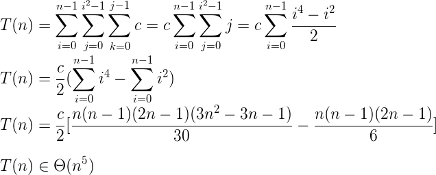
To find the exact area, you'd carry out steps 1-5 with a general $n$, use the closed-form summation formulas from earlier to simplify, and then take $\lim_{n \to \infty}$ of the result.