2.9 Calculus of the Hyperbolic Functions

Hyperbolic Functions

Hyperbolic functions are built from combinations of $e^x$ and $e^{-x}$. They show up frequently in integration problems and model real-world phenomena like hanging cables and signal processing curves. Their derivatives and integrals follow clean patterns that mirror (but don't exactly copy) the trig functions you already know.

Inverse hyperbolic functions reverse this process, and their derivatives produce expressions involving $\frac{1}{\sqrt{x^2 \pm 1}}$ and $\frac{1}{1 - x^2}$. These are particularly useful because they give you closed-form antiderivatives for integrals that would otherwise be difficult to evaluate.

Hyperbolic Functions

Applications of hyperbolic derivatives and integrals

The three core hyperbolic functions are all defined in terms of $e^x$:

• Hyperbolic sine: $\sinh x = \frac{e^x - e^{-x}}{2}$
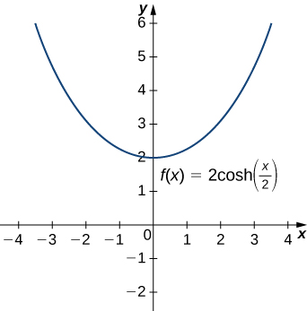
• Hyperbolic cosine: $\cosh x = \frac{e^x + e^{-x}}{2}$
• Hyperbolic tangent: $\tanh x = \frac{\sinh x}{\cosh x} = \frac{e^x - e^{-x}}{e^x + e^{-x}}$

Notice that $\sinh x$ is an odd function (symmetric about the origin) while $\cosh x$ is an even function (symmetric about the y-axis, always $\geq 1$). The graph of $\tanh x$ is S-shaped (sigmoidal), approaching $-1$ and $1$ as horizontal asymptotes.

Derivatives of hyperbolic functions follow patterns similar to trig derivatives, but without the sign changes:

• $\frac{d}{dx} \sinh x = \cosh x$
• $\frac{d}{dx} \cosh x = \sinh x$ (compare: $\frac{d}{dx} \cos x = -\sin x$, but here there's no negative sign)
• $\frac{d}{dx} \tanh x = \operatorname{sech}^2 x = \frac{1}{\cosh^2 x}$

Integrals follow directly from the derivative rules:

• $\int \sinh x \, dx = \cosh x + C$
• $\int \cosh x \, dx = \sinh x + C$
• $\int \tanh x \, dx = \ln(\cosh x) + C$
• $\int \operatorname{sech}^2 x \, dx = \tanh x + C$

The $\tanh x$ integral is worth remembering on its own. You can derive it by rewriting $\tanh x = \frac{\sinh x}{\cosh x}$ and using a $u$-substitution with $u = \cosh x$.

Inverse hyperbolic functions in calculus

Each inverse hyperbolic function can be written as a logarithmic expression, since the hyperbolic functions are built from exponentials:

• $\sinh^{-1} x = \ln(x + \sqrt{x^2 + 1})$, defined for all real $x$
• $\cosh^{-1} x = \ln(x + \sqrt{x^2 - 1})$, defined for $x \geq 1$
• $\tanh^{-1} x = \frac{1}{2} \ln\!\left(\frac{1+x}{1-x}\right)$, defined for $|x| < 1$

You don't need to memorize the logarithmic forms for most Calc II work, but you do need the derivatives:

• $\frac{d}{dx} \sinh^{-1} x = \frac{1}{\sqrt{x^2 + 1}}$
• $\frac{d}{dx} \cosh^{-1} x = \frac{1}{\sqrt{x^2 - 1}}, \quad x > 1$
• $\frac{d}{dx} \tanh^{-1} x = \frac{1}{1 - x^2}, \quad |x| < 1$

These derivative formulas are important because they tell you how to evaluate certain integrals directly. Compare them to the inverse trig derivatives you already know: $\frac{d}{dx} \sin^{-1} x = \frac{1}{\sqrt{1 - x^2}}$. The difference in signs under the radical ($x^2 + 1$ vs. $1 - x^2$) determines whether you get an inverse hyperbolic or inverse trig result.

Integration using hyperbolic substitution simplifies three standard integral forms:

1. For $\int \frac{1}{\sqrt{a^2 + x^2}} \, dx$, substitute $x = a \sinh \theta$. This gives $\sinh^{-1}\!\left(\frac{x}{a}\right) + C$.

2. For $\int \frac{1}{\sqrt{x^2 - a^2}} \, dx$, substitute $x = a \cosh \theta$. This gives $\cosh^{-1}\!\left(\frac{x}{a}\right) + C$.

3. For $\int \frac{1}{a^2 - x^2} \, dx$, substitute $x = a \tanh \theta$. This gives $\frac{1}{a}\tanh^{-1}\!\left(\frac{x}{a}\right) + C$ (when $|x| < a$).

These substitutions work because the hyperbolic identities $\cosh^2 \theta - \sinh^2 \theta = 1$ and $1 - \tanh^2 \theta = \operatorname{sech}^2 \theta$ clean up the expressions under the radical, much like trig substitution does for $\sqrt{a^2 - x^2}$.

Applications of Hyperbolic Functions

Catenary curves in engineering

A catenary is the curve formed by a uniform chain or cable hanging freely under its own weight between two fixed points. Its equation is:

$y = a \cosh\!\left(\frac{x}{a}\right)$

where $a$ is a constant determined by the ratio of cable tension to the cable's weight per unit length. This shape minimizes the potential energy of the system, producing a stable equilibrium.

Where catenaries appear in practice:

• Catenary arches and bridges: The inverted catenary shape minimizes bending moments in an arch, allowing thinner, more efficient structures. The Gateway Arch in St. Louis is a famous example. The Alamillo Bridge in Seville also uses catenary geometry to span large distances with less material.
• Suspension bridge cables: The main cables of a suspension bridge hang under gravity and approximate a catenary when supporting only their own weight. (Under a uniform deck load, the shape is actually a parabola, but the catenary model is the starting point for analysis.)
• Power lines: Transmission lines between towers form catenary curves. Engineers use the catenary equation to calculate required tower heights and maximum span lengths so lines don't sag too close to the ground.

Advanced Applications and Connections

• Hyperbolic geometry provides an alternative to Euclidean geometry and plays a role in Einstein's special relativity, where hyperbolic functions describe relationships between velocity, time dilation, and rapidity.
• Connection to complex numbers: Through Euler's formula, hyperbolic and trigonometric functions are related: $\cosh(ix) = \cos x$ and $\sinh(ix) = i\sin x$. This is why their derivative and integral patterns look so similar.
• Differential equations: Hyperbolic functions frequently appear as solutions to second-order linear ODEs, particularly those of the form $y'' - y = 0$, where the general solution is $y = C_1 \cosh x + C_2 \sinh x$.