1.2 The Definite Integral

The Definite Integral

Components of definite integrals

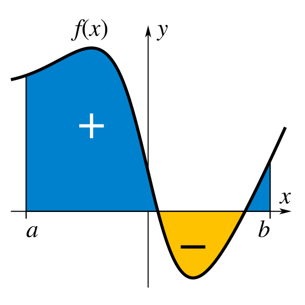
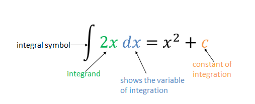
The notation $\int_a^b f(x)\, dx$ represents the signed area between the curve $y = f(x)$ and the $x$-axis over the interval from $x = a$ to $x = b$. Each piece of this notation has a specific meaning:

• Integrand $f(x)$: the function being integrated
• Lower limit $a$: the starting point of the interval
• Upper limit $b$: the endpoint of the interval
• Differential $dx$: tells you the variable of integration

The word "signed" is doing real work here. Regions where the curve sits above the $x$-axis contribute positive area, while regions below the $x$-axis contribute negative area. This means a definite integral can come out to zero if the positive and negative regions cancel, even when there's clearly area between the curve and the axis.

Integrability of functions

A function $f(x)$ is integrable on $[a, b]$ if the definite integral $\int_a^b f(x)\, dx$ exists and has a finite value. For that to happen, the function needs to be bounded on the interval, meaning there exist values $m$ and $M$ such that $m \leq f(x) \leq M$ for all $x$ in $[a, b]$.

The most useful fact here: if $f(x)$ is continuous on $[a, b]$, then it's guaranteed to be integrable. Functions with a finite number of jump discontinuities are also integrable, but continuous functions are the cleanest case.

Definite integrals as net area

The definite integral $\int_a^b f(x)\, dx$ computes the net area, not the total area. The distinction matters:

• If $f(x) \geq 0$ on the whole interval, the integral equals the geometric area under the curve.
• If $f(x) \leq 0$ on the whole interval, the integral equals the negative of the geometric area between the curve and the axis.
• If $f(x)$ crosses the $x$-axis, the integral adds the positive pieces and subtracts the negative pieces.

For example, if the area above the axis is 7 and the area below is 3, the definite integral gives $7 - 3 = 4$. If you wanted the total area instead, you'd need $\int_a^b |f(x)|\, dx$, which is $7 + 3 = 10$.

Riemann sums and the limit process

Definite integrals are formally defined as the limit of Riemann sums. The idea is to approximate the area with rectangles and then make the approximation exact:

1. Partition the interval $[a, b]$ into $n$ subintervals, each of width $\Delta x = \frac{b - a}{n}$.

2. Choose a sample point $x_i^*$ in each subinterval (left endpoint, right endpoint, or midpoint are common choices).

3. Build rectangles with height $f(x_i^*)$ and width $\Delta x$. The Riemann sum is $\sum_{i=1}^{n} f(x_i^*)\, \Delta x$.

4. Take the limit as $n \to \infty$. The Riemann sum converges to the definite integral:

$\int_a^b f(x)\, dx = \lim_{n \to \infty} \sum_{i=1}^{n} f(x_i^*)\, \Delta x$

This is the formal foundation. In practice you won't compute most integrals this way, but understanding the limit process helps you see why integration works as accumulation of infinitely many infinitesimal quantities.

Evaluating and Applying the Definite Integral

Techniques for evaluating definite integrals

Symmetry shortcuts can save you significant work when the limits are symmetric around zero (i.e., $[-a, a]$):

• Even functions satisfy $f(-x) = f(x)$. Their graphs are symmetric about the $y$-axis, so: $\int_{-a}^{a} f(x)\, dx = 2\int_0^{a} f(x)\, dx$
• Odd functions satisfy $f(-x) = -f(x)$. The positive and negative halves cancel exactly: $\int_{-a}^{a} f(x)\, dx = 0$

For example, $\int_{-3}^{3} x^3\, dx = 0$ immediately because $x^3$ is odd.

Core integration rules you'll use constantly:

1. Linearity: Constants factor out and integrals split over sums. $\int_a^b [c_1 f(x) + c_2 g(x)]\, dx = c_1 \int_a^b f(x)\, dx + c_2 \int_a^b g(x)\, dx$

2. Additivity over intervals: You can split an integral at any intermediate point $c$. $\int_a^b f(x)\, dx + \int_b^c f(x)\, dx = \int_a^c f(x)\, dx$

3. Fundamental Theorem of Calculus (Part 2): If $F'(x) = f(x)$, then: $\int_a^b f(x)\, dx = F(b) - F(a)$

This is the result that connects derivatives and integrals. Instead of computing a limit of Riemann sums, you find an antiderivative $F$, plug in the limits, and subtract.

Two additional properties worth knowing:

• Reversing limits flips the sign: $\int_a^b f(x)\, dx = -\int_b^a f(x)\, dx$
• Equal limits give zero: $\int_a^a f(x)\, dx = 0$

Average value through definite integrals

The average value of $f(x)$ on $[a, b]$ is:

$f_{\text{avg}} = \frac{1}{b - a} \int_a^b f(x)\, dx$

Think of it this way: you're finding the height of a single rectangle that has the same base $[a, b]$ and the same area as the region under the curve. That rectangle's height is the average value.

For a concrete example, if a car's velocity is given by $v(t)$ over $[0, 10]$, then $\frac{1}{10}\int_0^{10} v(t)\, dt$ gives the average velocity over those 10 seconds.

Applications of definite integrals

Definite integrals show up across many fields because they all involve accumulating a quantity over an interval. Common applications include:

• Area between curves: Integrate the difference of two functions over the region where one lies above the other.
• Volume of solids of revolution: Rotate a region about an axis and use disk, washer, or shell methods.
• Arc length: Compute the distance along a curve using $\int_a^b \sqrt{1 + [f'(x)]^2}\, dx$.
• Work: When force varies with position, $W = \int_a^b F(x)\, dx$.
• Moments and centers of mass: Use integrals to account for how mass is distributed.
• Probability: For continuous random variables, probabilities are areas under density curves.

When setting up any application problem, follow these steps:

1. Identify the quantity being accumulated and the relevant function.
2. Determine the correct limits of integration.
3. Write the integral expression that matches the problem's geometry or physics.
4. Evaluate the integral.
5. Interpret the result with appropriate units and context.