7.1 Parametric Equations

Parametric Equations

Parametric equations describe curves by expressing both $x$ and $y$ as separate functions of an independent parameter, usually $t$. Instead of writing $y$ directly as a function of $x$, you let both coordinates change with $t$, which makes it possible to represent curves that loop, backtrack, or trace complex paths. This is especially useful for modeling motion, where $t$ often represents time.

Plotting Parametric Curves

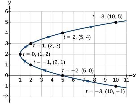
A parametric curve is defined by a pair of functions $x(t)$ and $y(t)$. As $t$ varies over some interval, the point $(x(t), y(t))$ traces out a curve in the $xy$-plane.

To plot a parametric curve:

1. Choose a range of $t$ values (for example, $0 \leq t \leq 2\pi$).
2. Evaluate $x(t)$ and $y(t)$ at several values of $t$ to get $(x, y)$ coordinate pairs.
3. Plot those points on the coordinate plane and connect them in order of increasing $t$.

The direction you connect the points matters. The curve has an orientation determined by the direction of increasing $t$, which you can indicate with arrows.

• Circle: $x = \cos(t)$, $y = \sin(t)$, $0 \leq t \leq 2\pi$ traces the unit circle counterclockwise starting at $(1, 0)$.
• Spiral: $x = t\cos(t)$, $y = t\sin(t)$, $0 \leq t \leq 4\pi$ traces a spiral that moves outward from the origin as $t$ increases, since the factor of $t$ grows the radius over time.

Conversion to Rectangular Form

Converting parametric equations to rectangular form means eliminating the parameter $t$ to get a single equation relating $x$ and $y$. This can help you recognize what type of curve you're dealing with (a line, ellipse, parabola, etc.).

Common elimination strategies:

• Solve and substitute: Solve one parametric equation for $t$, then plug that expression into the other equation.
• Use trig identities: When $x$ and $y$ involve $\sin(t)$ and $\cos(t)$, the Pythagorean identity $\sin^2(t) + \cos^2(t) = 1$ is your best friend.
• Algebraic manipulation: Square, add, or rearrange the equations to cancel $t$.

Example: Convert $x = 2\cos(t)$, $y = 3\sin(t)$ to rectangular form.

1. Isolate the trig functions: $\cos(t) = \frac{x}{2}$, $\sin(t) = \frac{y}{3}$.
2. Apply the Pythagorean identity: $\cos^2(t) + \sin^2(t) = 1$.
3. Substitute: $\frac{x^2}{4} + \frac{y^2}{9} = 1$.

This is the equation of an ellipse with semi-major axis 3 (along $y$) and semi-minor axis 2 (along $x$).

One thing to watch: the rectangular form sometimes includes more of the curve than the parametric version traces. Always check whether the parametric equations restrict the domain (for instance, only tracing the top half of an ellipse).

Parametric Equations for Basic Shapes

Lines:

A parametric line through the point $(a, c)$ with direction vector $\langle b, d \rangle$ is written as:

$x = a + bt, \quad y = c + dt$

The slope of this line is $\frac{d}{b}$ (provided $b \neq 0$). For example, $x = 1 + 2t$, $y = 3 + 4t$ passes through $(1, 3)$ with slope $\frac{4}{2} = 2$. You can verify by eliminating $t$: solving the first equation gives $t = \frac{x - 1}{2}$, and substituting into the second gives $y = 2x + 1$.

Circles:

A circle with center $(h, k)$ and radius $r$ has parametric equations:

$x = h + r\cos(t), \quad y = k + r\sin(t), \quad 0 \leq t \leq 2\pi$

Here $t$ represents the angle measured from the positive $x$-direction. For example, $x = 2 + 3\cos(t)$, $y = 1 + 3\sin(t)$ traces a circle centered at $(2, 1)$ with radius 3. Changing the interval of $t$ lets you trace just an arc instead of the full circle.

Interpretation of Cycloid Equations

A cycloid is the curve traced by a point on the rim of a circle as that circle rolls along a straight line without slipping. Picture a reflector on a bicycle tire as the bike moves forward.

The parametric equations for a cycloid are:

$x = r(t - \sin(t)), \quad y = r(1 - \cos(t))$

where $r$ is the radius of the rolling circle and $t$ is the angle (in radians) through which the circle has rotated.

Key properties:

• The curve is periodic. Each full rotation ($t$ increases by $2\pi$) produces one arch.
• The $x$-coordinate advances by $2\pi r$ per arch, which equals the circumference of the rolling circle.
• The $y$-coordinate oscillates between $0$ (where the point touches the line) and $2r$ (the top of each arch).
• At the cusps (where $t$ is a multiple of $2\pi$), the point touches the ground and the curve has a sharp point.

Example: For $r = 2$, each arch spans $4\pi$ units horizontally, and the point rises to a maximum height of $4$.

Cycloids show up in physics: the brachistochrone problem asks for the curve of fastest descent between two points under gravity, and the answer is an inverted cycloid. They also appear in gear tooth design and pendulum clocks.

Motion Analysis with Parametric Equations

When $t$ represents time, parametric equations naturally describe the motion of an object. You can extract velocity, acceleration, and tangent line information directly from $x(t)$ and $y(t)$.

Velocity vector: The velocity at time $t$ is

$\vec{v}(t) = \langle x'(t),\, y'(t) \rangle$

This vector points in the direction of motion. Its magnitude, $\|\vec{v}(t)\| = \sqrt{[x'(t)]^2 + [y'(t)]^2}$, gives the speed of the object at that instant.

Acceleration vector: The acceleration is the derivative of velocity:

$\vec{a}(t) = \langle x''(t),\, y''(t) \rangle$

Tangent line slope: The slope of the tangent line to the curve at any point is found using the chain rule:

$\frac{dy}{dx} = \frac{dy/dt}{dx/dt}, \quad \text{provided } \frac{dx}{dt} \neq 0$

If $\frac{dx}{dt} = 0$ but $\frac{dy}{dt} \neq 0$, the tangent line is vertical. If both derivatives are zero simultaneously, you need further analysis (such as L'Hôpital's Rule or examining limits) to determine the behavior at that point.